In a nutshell

In this blog post (Part 4 of this series) we use Monte Carlo simulation to explore the range potential outcomes given assumed Capital Market Expectations, (risk tolerance and corresponding) Asset Allocation, in the context of personal circumstances (Age, Assets, Expenses, Other Lifetime Income sources and the resulting required withdrawal rate) and compare these with annuitization. A series of examples how to asses ability to bear risk, approaches to portfolio de-risking and comparing outcomes to an annuity in terms of income, residual assets and NPV at various ages in retirement.

This five part series on Annuity/Pension vs. Lump-Sum is composed of: Annuity/Pension vs. Lump-Sum- Part 1: Making the right decision for you which explores risks in retirement,  Annuity/Pension vs. Lump-Sum- Part 2: Drivers to and away from annuitization  focused on qualitative considerations toward the annuity/pension vs. lump-sum decision,  Annuity/Pension vs. Lump-Sum- Part 3: Quantitative considerations focused on quantitative considerations in the decision,  Annuity/Pension vs. Lump-Sum- Part 4: Monte Carlo simulation to explore retirement income trade-offs with and without annuitization where Monte Carlo simulation is used to explore the range potential outcomes given assumed Capital Market Expectations, (risk tolerance and corresponding) Asset Allocation, in the context of personal circumstances (Age, Assets, Expenses, Other Lifetime Income sources and the resulting required withdrawal rate) and compare these with annuitization. Then in order to help see the entire picture, in the 5^th and final part of this series  Annuity/Pension vs. Lump-sum- Part 5: Putting it all together  I use the case of an 85 year old single male with a life expectancy (i.e. 50^th percentile) of the order of 5 years and a 90^th percentile life expectancy of about 11 years, instead of the mostly used 67 year old couple who needed to finance a potentially 30 year long retirement.

 

 Note: You can click on any of the figures to enlarge them, then return to the blog post by clicking Back on the browser

Disclosure and warning

Note that none of what follows should be construed as advice on what you personally should do in your pension/annuity vs. lump-sum decision. Think of this as my (Peter’s) journey to such a decision (which it is) and feel free to consider this as only educational material on how one might go about examining such a decision in as informed manner as possible. There is no one universally right answer; what may be right for me might be completely wrong for you. The future is unknown and unknowable (as most of us found out in the fall/winter of 2008/9) and the lack of transparency of financial products in general and insurance products (like annuities) in particular, make the annuity vs. lump sum decision particularly difficult. Furthermore, limitations (cloudy crystal ball) of capital market expectations, models, assumptions, simulation approaches which are used to explore possible outcomes, will almost certainly insure that the future will not unfold as expected except by pure coincidence.  Unbiased professional advice (ideally with a fiduciary level of care) on such important decision is usually advisable. This further complicates matters because of potential conflicts of interest which burden many of those that you might approach for advice (from insurance salespersons who would benefit from selling you an annuity, all the way to advisors under pressure to accumulate assets under management (AUM) from which they generate fees). So keeping in mind that I am not an actuary, that there is potential for errors on my part, and that your personal circumstances/perspectives, may be radically different than mine, are ultimately the primary drivers to the decision.

 

Context

A 67 year old couple

Joint Life Expectancy (general population) percentiles: Approximate 50^th=23, 75^th= 27, 90^th=31 years corresponding to ages 90, 94 and 98 respectively. The annuitant table life expectancy (50^th percentile) =25 years, or age 92

Joint Annuity Rate=6%

Planning horizon= 27 years/age 94 at 75^th percentile life expectancy, and (up to) 28 and 33 years (if we choose ages 95 and 100)

Part of the Context for this 67 year old couple are two important pieces of information: (1) the Expenses: Fixed and discretionary, and (2) the current Capital Market Expectations which is an educated guesstimate of what returns and corresponding risk is likely over the decade.

 

In the Canadian context, in PWL Capital’s “Great Expectations- How to estimate future stock and bond returns when creating a financial plan” Kerzeho and Bortolotti consider explicitly Canadian Capital Market Expectations, in context of a Canadian investor’s portfolio for which they define their stock allocation as 1/3 each of the Canadian, U.S. and International stocks while the bond allocation is 100% Canadian. For a 60/40 stock/bond portfolio the Capital Market Expectation is given as Return=5.8% while the Standard Deviation=7.8% (as compared to Vanguard’s American investor portfolio allocation for a 60/40 mix a same ballpark Return=6.25% and but significantly different SD=11.2%).

 

A Systematic Withdrawal Strategy- Proportional with Ceiling and Floor

The systematic withdrawal approach involves:

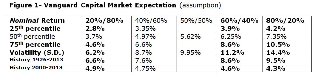
-selecting a (risk tolerance compatible) asset allocation for retirement portfolio (asset allocation will be transformed into a normally distributed portfolio with specified parameters of expected ‘Return’ and ‘Standard Deviation’; the Monte Carlo simulation involves generating a large number of returns from the distribution (the parameters for the normal distribution are discussed in the Vanguard Capital Market Expectations section of Part 3 and reproduced above in Figure 1)

-identifying all lifetime income sources (government and company pensions, and any pre-existing annuities), you might even want to subtract all other lifetime income sources from the expenses, and just enter the (Net) Expenses. For lifetime income streams not indexed for inflation it might make sense to de-rate them to about an average of 80% over a 25-30 year retirement to account for expected purchasing power drop with time.

-determining our total expenses per year during retirement (see the Expenses: fixed and discretionary section of Part 3)

-running Monte Carlo simulation using a withdrawal rate (%) necessary to meet specified initial expenses (calculated automatically from Assets, Expenses and Other Income you have entered)

-“Proportional” withdrawal strategy draws the same percent from the portfolio each subsequent year but the dollars drawn are based on previous year’s year-end value of portfolio; this is to recognize the reality that humans are adaptable and will respond to poor market performance by reducing spending (Note that after a 10% drop in portfolio value, this proportional method would result in 10% drop in income the following year)

-“Ceiling-and-floor” is a mechanism used with the “proportional” withdrawal strategy to moderate the year-to-year changes in income (as described in Jaconetti and Kinniry’s Vanguard article) by adding the “Ceiling-and-Floor” parameters which specify the maximum and minimum allowable upward and downward annual income adjustment (in our examples we’ll set Ceiling at 5% and Floor at -2%, but this is a user input so you can change at will)

-Note that while it is near impossible  to run out of money with a pure “proportional” strategy (it could happen if you had 100% in equities and the market went to zero), since one is drawing each year some small percent of available assets, one could end up with such a low income level that it would feel essentially the same as having run out of money; however with the added “ceiling-and-floor” constraints as some of the examples will show, it is actually possible to run out of money.

-All the simulations assume that you are a do-it-yourself investor and the portfolio is implemented with very low cost passive index funds so costs/fees are effectively set to zero. To factor in the effect of fees, just subtract the percent cost from the return in the simulation (i.e. if Capital Market Expectations are for a return of 6.25% and you are paying 2% fees, then all you have to do is reduce 6.25% input return to 4.25% and run simulation again.)

 

Monte Carlo simulation

Keeping in mind that the future is unpredictable, we not only can’t predict with confidence the market returns over the next 10-years, but we also don’t have a really good model for the statistics of return distributions; so we’ll assume that normal distributions with the parameters indicated in Figure 1– Vanguard Capital Market Expectations above.

We will use these parameters, for the normal distributions corresponding to the indicated asset allocations, to explore the potential outcomes under different combinations of lifetime income, portfolio size/allocation and required income to meet expenses. This is typically referred to as a form of systematic withdrawal plan. In this case, we’ll do a Monte Carlo simulation which assumes a proportional withdrawal strategy whereby the dollar value of the withdrawal each year will be a specified percent of the remaining portfolio assets at the end of the previous year. That specified percent is determined by the initial (pre-tax) income required to meet Total expenses. So as the portfolio is reduced by losses and/or withdrawal, the dollar withdrawals (and our lifestyle) are also correspondingly reduced. In order to contain the year-to-year income variability due to changing portfolio assets, we’ll also constrain allowable income changes to have 5% ceiling and a -2% floor on a year-to-year basis. (If you want to try  a pure proportional withdrawal strategy, all you need to do is replace the ceiling and floor values with a large and small number, e.g.  +75 and -75.)

We’ll then compare these outcomes as we create scenarios of varying mix of annuity/pension vs. asset values (Note that the dashed black self-annuitization lines (income and NPV) do not include the pre-existing pension/annuity specified as input, whereas the SPIA (annuity) line includes these.). We could explore how long we’d be able to draw the same income stream as offered by pension/annuity before we run out of assets in the portfolio. We’ll also have the option to compare the annuity offered with the one we’d be able to get on the market by going to a mortgage broker to get the ‘best’ available annuity rates (quoted a dollars of monthly income for a $100,000 annuity premium) from the market or by looking at  the Globe Investor/Markets available weekly annuity rates compiled by Cannex and some U.S. rates at ImmediateAnnuities.com which were shown in Figure 6 Part 3; in the same blog posts you can find Figure 7 Self-Annuitization rates.

Examples: Exploring a systematic withdrawal alternative to annuities?

Instead of locking in a 2.5% interest rate for life (even if boosted by mortality credits which come with longevity risk pooling), we will now examine what happens if one has higher risk tolerance and would be able to invest in a mix of stocks and bonds instead of annuitizing.

We just have to remember at all times the mathematician Richard Hamming’s admonition that “computing is for insight, not numbers”. i.e. this is not about believing that the specific outcomes will actually happen, but more about exploring the ranges and likelihoods of possible outcomes, so we gain the necessary insight on the advantages/disadvantages of various scenarios. Many of these simulations cover 25-35 year sequences, but we can declare any point in time as time=0 and reset our strategy and rerun the simulations with or without changes in assumptions.

So let’s see where this takes us.

Self-Annuitization rates (at 2.5% average risk-free intermediate/long-term interest rate) are 5.01%, 4.89% and 4.38% at ages 94 (75^th percentile joint life expectancy), 95 and 100 respectively

Initial Asset Allocation is 60%stock/40%bond with Capital Market Expectation of Return=6.25%, S.D. =11.2% (from Capital Market Expectation table above)

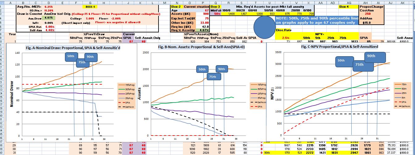
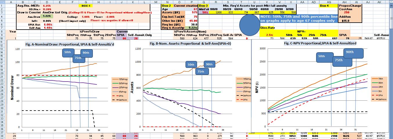
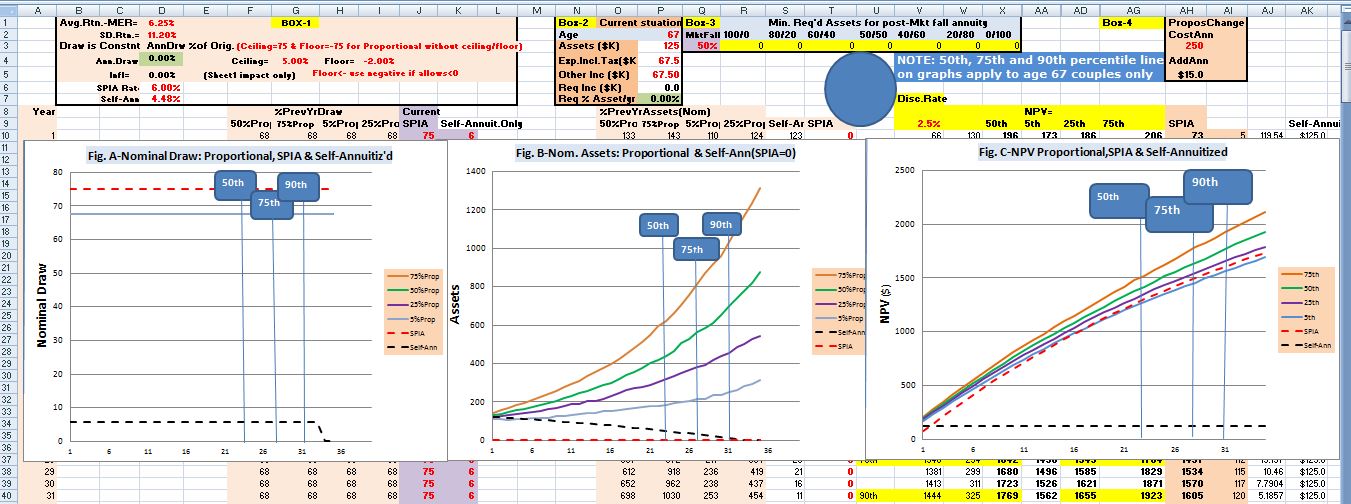
In each example the Monte Carlo simulation results are plotted on three graphs:

-Fig. A represents “nominal income” (Draw),

-Fig. B represents remaining “nominal assets”, and

-Fig. C represents Net Present Value (NPV) at any point in time should death occur that year.

On each graph 75^th, 50^th, 25^th and 5^th percentile outcome curves are displayed in solid brown, green, purple and blue lines respectively, while dashed lines indicate corresponding annuitized and self-annuitized results, in red and black respectively. Note that 50^th percentile represents most likely outcome as half the outcomes are higher and half lower than the 50^th percentile by definition; the 75^th percentile indicates that 25% of the outcomes are higher, while the 5^th percentile that 5% of the outcomes are lower (and we don’t know how much lower).

Again, note that none of the self-annuitization lines (Draw, Assets or NPV) on the graphs (the black dashed line) include the value of the pre-existing $15K annuity indicated in the example, however that pre-existing annuity is included in both the annuity and systematic withdrawal curves.

 

Illustrative Examples

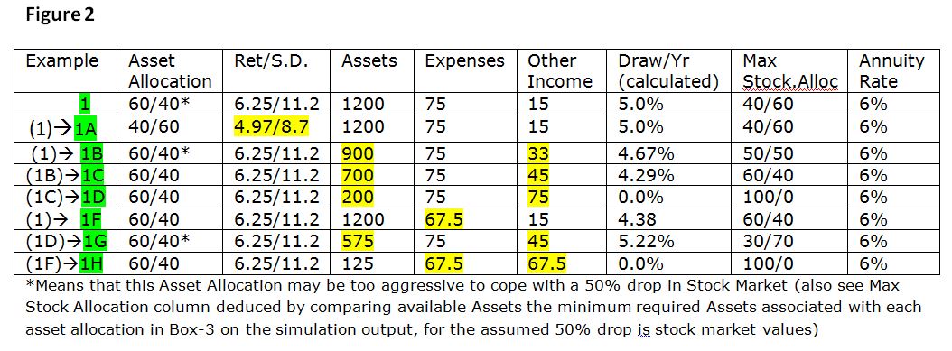
Starting with a base case we step through a series of examples to demonstrate how to asses maximum tolerable risk as measured by maximum stock allocation and explore various de-risking strategies and compare outcomes with annuities in terms of income, remaining assets and net present value (NPV) at various ages throughout retirement. As we discussed in earlier blog posts since annuitization just trades-off longevity risk for inflation risk, another measure of goodness of a solution is if at least the median income in retirement is increasing over time to even partially compensate for inflation. De-risking strategies include: lowering stock allocation in the portfolio, reducing expenses (and withdrawal rate), doing partial or complete annuitization, and/or some combination of these.

The table in Figure 2 below shows the various scenarios that we’ll be discussing, the first one being the base case, while the following ones show the highlighted in yellow) input changes that were made from example to example:

 

The link to the Monte Carlo simulation spreadsheet is available at http://1drv.ms/1pZoseS  but to execute this macro based spreadsheet you’ll have to open it in Excel and run it locally on your computer. To do this in Excel 2007: click on the link, then in Online Excel: Go to File, Save As, Download a Copy, and then Open (which will open it in the Excel application on your computer. To enable macro you’ll have to Click on “Options”   (just above the spreadsheet) then click on “Enable the macro”, and to run example once you have specified the inputs, you’ll have to click on the large Blue button. To do this in Excel 2010: Enable editing (disabled for security reasons), Enable content/macros (disabled for security reasons), Make macro visible under tab View/Macros/View Macros (The name of the Macro is CalcNow_Click)

Also note that items shown in red font are the only permissible inputs.

 

Example #1

Pre-tax income requirement:

-Total=$75K, comprised of Fixed/Musts=$55K and Variable/Wants=$20K

Other Lifetime income=$15K (government pensions)

Assets=1200K

Required income to meet Total=$75K less $15K existing lifetime income, leaves $60K of income to be generated or as shown in the spreadsheet (green background) 5% of the $1200K assets.

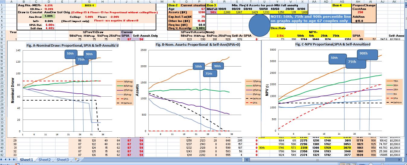
Simulation results show:

-Annuitizing the entire $1200K would deliver a lifetime income $87K (including $15K from other sources) exceeding the required $75K/year, and there would be no residual capital left. This is not something that most people would even contemplate

-the 50^th percentile (median) outcome starts at the required $75K (including the $15K pre-existing lifetime income) and increases by life expectancy point at age 90 to about $87K, but still leaves expected (50^th percentile) residual assets about 10% higher than the $1200 we started with (i.e. met our needs AND kept the money we started with)

-the 5^th percentile income line starts at $75K and falls about 30% to $53K by age 90 (the 50^th percentile), which is close to the Fixed/Musts expenses of $55K, but assets dropped now  to $220K, and of course the effect of inflation will further erode buying power (similar to annuity income). Clearly many might not just continue spending at the same rate until age 90, but would likely take some earlier corrective action

-Stress test: Do we have an annuity fallback option should there be an immediate 50% drop in the market (leading to a 30% drop in assets) for a 60/40 portfolio? No, because Box 3 (top 3 lines of spreadsheet indicates that $1429K would be required (so that $1000K would still be left after a 30% asset drop). We are only protected against a 30% immediate market drop. Instead we’d have to reduce asset allocation to about 40/60 which would get us close to the $1200K requirement (We’ll re-run simulation shortly).

-NPV perspective: note that the annuity NPV is always lower than median (50^th percentile) systematic withdrawal NPV over the planning horizon, and $700K lower at life-expectancy. The 75^th percentile line NPV is >$1500K higher than annuity NPV over entire planning horizon, while the annuity NPV crosses over the 5^th percentile line after about 17 years (joint age 84) and the 25^th percentile line just past life expectancy (23 years).

Risk management approaches to dealing with Stress test results in Example 1 could be either reducing stock allocation or annuitizing some of the assets or reducing expenses. We will explore these various approaches of risk reduction, and we’ll observe to what extent we can also achieve some inflation mitigation, increased residual assets and/or higher NPV compared to annuitization:

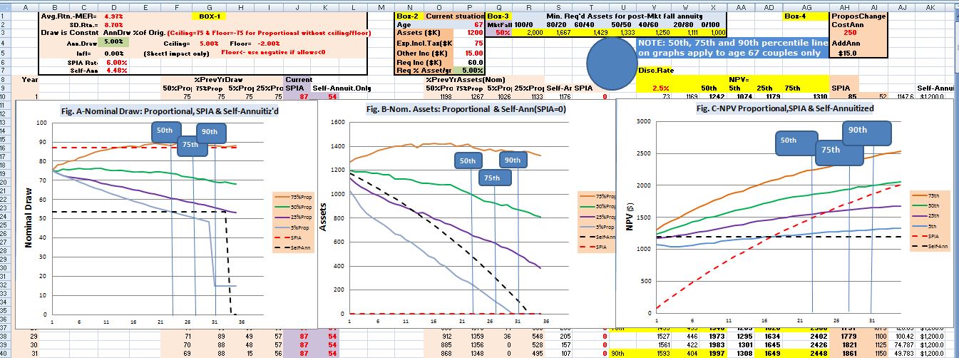
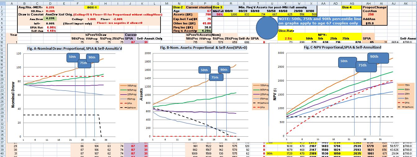
Example 1A (reducing risk by lowering stock allocation) shows how the outcome changes when asset allocation to stocks is reduced from 60/40 (60% stock) to 40/60 (40% stock). This allocation can absorb close to the 50% drop in the stock market body blow and still have sufficient funds remaining to annuitize. However this puts us on a path of decreasing expected income and assets over time, due to expected returns dropping to 4.97% from 6.25% (from Figure 1).

 

Example 1B (de-risking by annuitizing part of the portfolio assets) also starts with the Example 1 asset allocation of 60/40, but this time instead of reducing stock allocation to reduce risk, we annuitize $300K (or 25%) of the existing assets. The outcome is shown below. Note that here expected income is increasing, but it is at the expense of immediate asset drop of $300K (perhaps a reasonable trade-off for some retirees) especially when you consider that NPVs are higher than in Example 1A. But note that we still don’t have the perhaps desired asset level to give us an annuity fallback option after a 50% stock market drop,

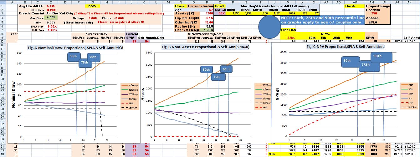
Example 1C (de-risking further by annuitizing a larger part of portfolio assets) looks at the scenario where we further increase the annuitized assets to $500K which now leave only assets of $700K, but this gets withdrawal rate to 4.29% and tightens the range of 5^th to 75^th percentile income outcomes, we also get upward slopping median income so we are buying some (about 0.65%/yr) inflation protection and we have enough assets remaining for downside protection that we can annuitize without loss of short-term buying power against a 50% market drop.

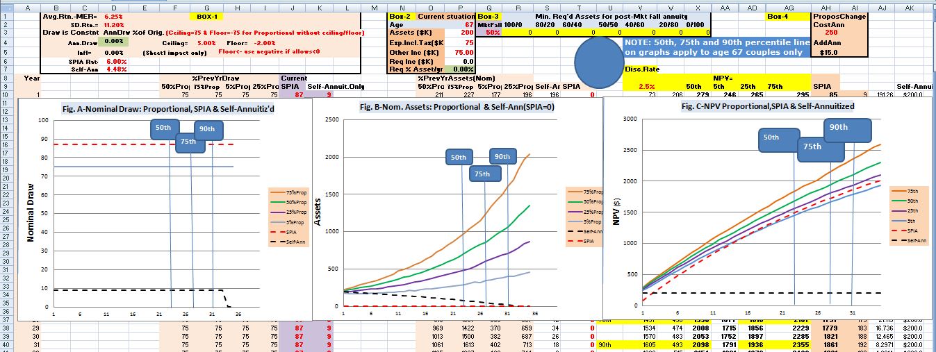
Example 1D (de-risking longevity risk completely by annuitizing enough assets to cover 100% of expenses on day 1) we show how we could annuitize (even more but) just enough to generate $60K (for a total income of $75K including $15K existing annuity) and we note here the assets rising from the initial $200K level at age 67 to about $300K/$500K/$700K/$1000K level on the 5^th /25^th /50^th /75^th percentile asset curves in 23 years by life expectancy at age 90. It’s actually a workable solution as we secured the initial requirements at least nominally, we’ll likely have sufficient assets to make gradual income adjustments to (at least partially) compensate for inflation and we have a substantial emergency/end-of-life-care/bequest pot

Example 1F (de-risking the base-case by reducing expenditures on day 1) is same as the starting Example 1 with the $1200k assets but we reduced expenses by 10% to $67.5K, so we only need $52.5K to cover expenses. Now expected income and assets gradually climb by age 90 (50^th percentile age) to about $82K and $1600K to allow to give more inflation compensation relative to starting income and a significant asset growth from $1200K to $1600K should we desire a larger estate, more emergency cash or even higher income. Also note that by reducing expenses from $75K to $67.5K we effectively increased our risk tolerance as measured by a “stock market drop of 50%” since now the 60/40 asset allocation case only needs $1250K rather than $1446K to withstand this shock and still deliver required annuity.

Example 1G (examines the case when cash value offered instead of annuity is lower than cost to purchase annuity, as implied by expected annuity rate) is the same as 1C, except when we started with 1D and working toward Example 1C instead of getting $500k back for giving up $30K annuity, we only get $375K to give up the $30K annuity (e.g. due to legislated cash-value adjustments as in the Nortel pensioners’ case). Clearly, not a very good deal.

 

Example 1H (de-risking portfolio by simultaneously reducing expenses and annuitizatizing enough assets to meet expenses on day 1) one can think of as starting from Example 1F but available assets are not $1200K but only $1000K, and suppose that we are able to reduce expenses by 10% to 67.5. Now let’s see the effect of generating $52.5K additional annuity, requiring $875K, to the pre-annuitized $15K, so we covered all expenses at retirement start with annuities. We then have $125K left from the $1000K which we can invest in a 60/40 portfolio from which no draw is required; so we have an opportunity to allow assets to build for emergency needs, some augmentation to mitigate inflation, and perhaps even leave some assets for the estate.

As you can see, while there are some un-controllables like: how long you are going to live, how much inflation headwind you’re going to face, what the stock market will do, whether you’ll suddenly need some emergency funds for a crisis; but whatever comes our way we’ll have to deal with. Then there are a few of moving parts that we can control to various degrees like: starting value of assets as we head toward retirement, spending/expenses, deciding to annuitize or not, how much to annuitize  and/or going with a systematic  withdrawal plan to meet our expenses, whether we would like to leave estate and what size are we aiming for, we must minimize investment management and advice costs (remember that we are approaching the problem with the expenses as the starting point and trying to secure the income to cover them as long as we live, rather than saying let’s try to maximize withdrawals without running out of money.)

 

Bottom Line

The decision of if and when to annuitize some or all the remaining assets can be reviewed periodically, or at a point of radical changes in assets or expenses due to unexpected external forces. One can also monitor which percentile is operational curve (in Fig. A and B on Monte Carlo simulations) for assets/income between major review points and determine what if any corrective action might be required.

As to pension/annuity vs. lump sum decision, it cannot be made in isolation of the total financial picture; one really must factor in other available resources, assets and lifetime income, so we have a holistic picture on whether one needs the insurance at any point in time.

So the Monte Carlo simulation will help us to get some insight on the quantitative trade-offs that we’ll be making toward the annuity/pension vs. lump-sum decision.