In a nutshell
The risk of outliving retirement savings is a persistent worry of those approaching or in retirement. A tool was built to help answer the “How much you can spend each year without running out of money?” question based on givens (age, assets, income/pension, risk-free rate and tax rate), maximum stock allocation (based on selected measures of objective risk-tolerance), minimum stock allocation (based on goals driven by desire for higher retirement income and/or residual estate), controllables (fixed and discretionary expenses, asset allocation guided by min/max stock allocation bounds) and a set of conservative assumptions for uncontrollables (market returns (RFR,ERP), inflation and plan horizon/longevity). The tool enables one to take an adaptive approach to spending and risk during retirement and can be re-run annually and/or following adverse market/spending events to reflect current reality. Each year is the first year of the remaining plan horizon, so it is adaptive and self-correcting by allowing one to adjust the controllables. The tool helps gain insight into the plan outcomes resulting from the complex interaction of the governing factors. (See May 1, 2018 note on correction at bottom of this post.)

Historical approach to decumulation
The risk of outliving retirement savings is a persistent worry of those approaching or in retirement. How much you can spend each year without running out of money (decumulation) is a much more difficult question than saving for retirement (accumulation), and the consequences of getting it wrong get more and more severe as ‘DB pensions’ are disappearing (See “Once upon a time” New Yorker cartoon)
I’ve been blogging on retirement finance education and advocacy for about a decade. On the advocacy front a lot of my focus has been on DB pensions and how to save/protect existing commitments or how to try to use pension-like products like immediate or deferred annuities (a.k.a. longevity insurance, i.e. products which deliver a lifetime income stream starting immediately or at some future age (e.g. 85).
In this blog post, instead of trying fix the systemic pension issues festering for decades and often unraveling/collapsing under the weight of boomer demographics, financial repression, increasing life expectancy and sponsor’s underfunding/mismanagement, we’ll dispense with pensions and annuities (other than as a comparative reference) and show how we can tackle the decumulation problem adaptively.
I was always fascinated by decumulation papers covering the interesting approaches to decumulation. The most famous and most persistent being William Bengen’s 4% rule, where it was postulated based on historical market returns, that one could draw from a balanced portfolio 4% (recently many suggest a safer 3%) of its initial value in year one and then increase draw annually by inflation without exhausting the portfolio over a 30-year retirement.
Concerned about using future returns based on past market returns, some suggested the use statistical distributions for expected future returns. Others, concerned that substantial portfolio losses early in retirement (e.g. sequence of return risk) combined with the increasing annual withdrawals might lead to portfolio exhaust before the assumed 30 year retirement, suggested using proportional withdrawal strategy where 4% of assets available each year could be withdrawn; others, to reduce income volatility, suggested a floor/ceiling enhancement of the 4% proportional rule such that in bad/good years one might limit withdrawal reductions/increases to no more than -3%/+5%. Many used Monte Carlo methods (running thousands of scenarios) to evaluate the probability of running out of money during retirement. Finding that ‘only’ 10 or 15% of the simulated scenarios resulted in a retirement failure, might be comforting to some, but I suspect most real retires would be uncomfortable with any set-and-forget approach over a 30 year retirement period which might lead to even a small probability of asset exhaust; and certainly most wouldn’t just continue spending at a the same rate after they saw their portfolio drop precipitously due to poor markets and excessive withdrawals based on portfolio size at start of retirement. Of course, with increasing life expectancy over past half century, planning for a 30-year retirement should make many 55-65-year-olds even more apprehensive.
The major risks in retirement finance are usually listed as: market risk, longevity risk and inflation risk.
Life expectancy (the median years of life remaining as any age) is clearly an unsuitable measure for retirement plan horizon. If a 65-year-old spends at a rate based on the assumption of dying at age 85 (life expectancy), he will have a very unpleasant(?) surprise if he should live to age 90, 95 or 100 and will have to become a burden on the state and/or his children. Waring and Siegel (which I discussed in “The only spending rule article you’ll ever need” by Waring and Siegel- A review) proposed a very simple approach to generating a conservative planning horizon for healthy individuals. They recognize that for healthy 65-year-olds using life expectancy as the planning age of death to be very risky, but at the same time using 120 (the current longest realistically expected lifespan) would result in an overly conservative a planning interval. So, they chose a (still) conservative planning age, plus eliminate inflation and market risk by investing into a laddered portfolio of TIPS STRIPS (inflation protected government bond STRIPS) matching the spending liability in each year maturing in one of the years covering the plan horizon calculated as above (average of life expectancy and 120). This approach, for a 65-year-old with a life expectancy of 85, yields a planning age (of death) of (85+120)/2= 102.5. As this individual ages by 1 year his life expectancy increases by somewhat less than 1 year; so, by the time such person becomes 85 their life expectancy might be 92 and resulting in an increase in the planning age to (92+120)/2= 106, whereas at age 92 the planning horizon would have increased to 108! For simplification, Waring and Siegel use an annuity calculation to determine how much one can spend each year, without actually buying an annuity; it is just a way of calculating the annuity payment if such a real annuity were purchased with the available funds at the current real annuity rates. This determines the maximum spend rate with this riskless approach.
Waring and Siegel hint how one might choose to use a risky portfolio, but they do not explicitly address risk tolerance, how fixed/discretionary spending might help to determine it, the corresponding stock allocation for the retirement portfolio and the maximum spend rate based on expected long-term return on risky assets. In this blog post and accompanying tool I tackle the risky portfolio extention to Waring and Siegel’s approach.

So how much can you spend in retirement?
In my 2015 blog post I included a spreadsheet which calculates not just stock allocation, but also how much can you spend in retirement; the spreadsheet in this post has simplified inner workings as well as enhanced capabilities. Since we are working with risky assets, we need to make some conservative assumptions over the planning horizon of the retiree under consideration about: average real return on risk-free assets (FRF), the equity risk premium (ERP) and inflation. We’ll also need to estimate fixed and discretionary expenses for the retiree, make some assumptions about maximum market drop scenarios for the risky portion of the retirement portfolio, based on which we can calculate the maximum stock allocation (an objective measure of risk tolerance) of the portfolio. Similarly, we can create lower bounds for the stock allocation required to achieve desired objectives and the minimum required stock allocations to achieve these. At the beginning of each year (or more frequently when massive market dislocation has occurred) we can repeat the calculation with current portfolio value, the current age (and retirement planning horizon) and any updates to latest market expectations. So, let’s look at the tool/spreadsheet.

Assumptions
-passive investment approach only, using current available average real RFR over plan horizon and an assumed conservative (by historical standards) real ERP; real return on equities is assumed to be “real RFR” + “real ERP”.
-for simplicity, female life expectancies are used by averaging them with 120 to calculate conservative plan horizons at each age, whether male/female/joint; conservative planning horizon (103 at age 65, 107 at 90) insures substantial reserves for: emergencies, late life increases in expenses (long-term care) or possibly even a bequest

The potential value of the tool is:
-not just overcoming the fear of running out of money before end-of-life, but finding the fine balance between, being an overly cautious spender (i.e. the old joke: “if you don’t travel first class, your children will”) versus being a spendthrift and damaging your (and potentially your children’s’) lifestyle/comfort in your later years
-to help find and adjust one’s spending by: adapting to changes in needs/wants (fixed/discretionary spending) each year, responding to adverse market events, decreasing plan horizons by less than a year as one ages each year, and inflation variations compared to plan
-to find the appropriate stock allocation for your portfolio guided by 8 criteria assessing your risk tolerance (maximum stock allocation) and your need to take risk to achieve desired goals (minimum stock allocation)
-helpful in managing sequence of return risk by containing objective risk level in terms of downside market risk (e.g. will I have sufficient remaining assets after an assumed market drop to continue spending at the planned rate for musts/wants based on investing only in risk-free assets like TIPS/RRBs) and/or offering a systematic approach to adapting (adjusting expenses) to adverse market/spending events; understanding objective risk tolerance helps manage subjective risk tolerance
-a mechanism to factor in the most important givens (age, assets and income), controllables (spending and asset-allocation) and uncontrollables (longevity, inflation and market risk) in the context of assumed Capital Market Expectations and tax rates when planning retirement spending to end-of-life…and then annual review a forward-looking plan rather rear mirror based wishful thinking
– useful for lay and expert users to annually (re-)plan spending during retirement given assets/income, spending need/wants, risk tolerance, without the need to understand spreadsheet details to get the spreadsheet benefit
– helpful in understanding the interplay between fixed/discretionary expenses, risk tolerance and downside market risk, as well as opportunity/need to assume risk to achieve certain objectives, and enhances ability to proactively plan for and respond to adverse market conditions by reducing/eliminating discretionary spending
-helpful in understanding when annuity might be required, the trade-offs between this adaptive approach and annuity (SPIA), the opportunity to understand and proactively deal with the corrosive effect of inflation, the higher probability of having residual assets for a bequest; the key metric for comparing the approaches is the Cumulative Real Benefit until Death for the Annuity (defined as the total real income received) versus the Adaptive approach (defined as the total real income until death plus real value of residual assets)
-helpful in understanding how to limit risk below recommended maximum to maintain reserves (keeping some powder dry) ready to invest at sale prices during a market correction

The tool/spreadsheet layout
This retirement planning tool/spreadsheet described here might first look daunting but is quite simple to use in reality; easily accessible to expert and lay users.
There are three color highlighted sections (‘green’, ‘yellow’ and ‘blue’) where required and default inputs in red font are highlighted, as well some corresponding key outputs are shown in the same color; if an annuity option is being considered a ‘pink’ highlighted annual Annuity/$1000. input is required. ONLY cells in red font can be modified; other cells must not be changed. There is also a graphical section showing assets and draw over time corresponding to a given set of inputs/assumptions. The model assumes a two-asset class portfolio composed of a risk-free and a risky/stock component. The resulting plan covers the entire plan horizon until death, but it is recommended that the plan should be rerun at least annually and following a significant market event (e.g. >20% market dip), to reflect changes. Referring to Fig 1 (below) or by opening the tool:
(i) In the ‘green’ portion of the spreadsheet you must specify the retiree’s circumstances: age, pension/income, assets and average tax-rate from which the MaxDraw/yr (maximum withdrawal permitted per year) can be calculated assuming initially that portfolio is built comprised risk-free assets (0% Stock allocation). A conservative Plan Horizon is also calculated as the average of female life expectancy at any age and 120 (considered the maximum lifespan at this time) as proposed by W-S. You must also define your Total Expenses specifying your Fixed Expenses (Musts), two types of Discretionary Expenses (Wants) Level 1 (L1) which might take a couple years to shed (e.g. a second home) and Level 2 (L2) which can be shed immediately (e.g. travel/vacation/restaurants/entertainment); Expenses are specified net-of-tax (i.e. after tax paid) and Total Expenses= Fixed+ L1+ L2. The Maximum and Minimum stock allocations are also shown in the ‘green’ section based on the 8 listed guiding criteria
(ii) The ‘yellow’ portion spreadsheet provides the modifiable conservative default Capital Market Expectations (CME) (e.g. Real Risk-Free Rate, Equity Risk Premium (ERP) and Inflation; inflation is only used in the graphs to illustrate the Nominal Assets and Draws over the plan horizon. In this ‘yellow’ section the default market drop is set to (a modifiable) ‘50%’ to calculate the maximum stock allocation permitted to be able to tolerate such a 50% drop and still have sufficient assets remaining to protect the specified spending level of Fixed+ L1 over the Plan Horizon using a portfolio of Risk-Free Assets. In addition, one can also specify market drop scenarios of any size during the 2nd year of the plan and see graphically the impact on Assets and Draw.
(iii) In the ‘blue’ portion of the spreadsheet one can select/specify an acceptable portfolio ‘Stock Allocation’ based on the Maximum permitted and Minimum required Stock Allocations from the 8 criteria; from the specified Stock Allocation corresponding ‘MaxDraw/yr”’ (maximum permitted draw per year) is calculated.
(iv) If an annuity comparison is desired, then the Annuity/$1000 input is required in the ‘pink’ highlighted section.

An example
Base case spreadsheet data is shown in Fig 1 (below)

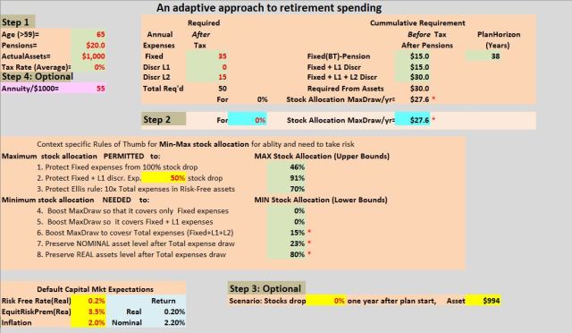
Fig 1 Base case data

Fig 2 shows graphical output corresponding to Fig 1 Base case spreadsheet data. The red line in the left two graphs of (Draw and Cumulative benefit at Death) show an immediate Annuity (SPIA) purchased with the assets compared to this Adaptive approach shown in the blue line. The right-most graph shows Draw and Assets in real and nominal dollars for the Base case. Observations: (1) this is a very conservative scenario of risk-free portfolio with real return of 0.2%/yr, (2) still, the nominal draw stays above the starting value until well over age 100, (3) while the real annuity income is higher until age 120, the cumulative real benefit of the Adaptive>Annuity until about the life expectancy (age 85) of this 65 year old, (4) we also note that a the Fixed expenses would be protected even if the value of the stocks dropped 100% to zero if we increased stock allocation to the maximum permissible value of 46%, (5) but the required income ($30K) from assets is greater than maximum permissible draw ($27.6) from this risk-free portfolio

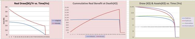
Fig 2 X=0% Base case Stock Allocation=0%, i.e. entire portfolio is risk-free

Although as little as only 15% stock allocation would sufficient to cover Total expenses (per Criterion 6), we choose to increase the stock allocation to the maximum permissible 46% (per Criterion 1). Fig 3 below shows the result graphically. Observations: (1) the right-most graph indicated that the nominal draw and assets are respectively increasing and constant until over age 100, (2) but the real draw of annuity exceeds the income specified or desired in the Adaptive approach over most of the plan horizon, (3) however the cumulative real benefit of the Adaptive approach is higher than that of the annuity if death occurs before age 100, even with the very conservative default Capital Market Expectations

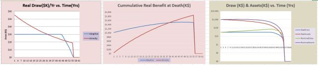
Fig 3 X=46% Req’d income> MaxDraw of risk-free portfolio, Stock Allocation is set to Max permitted and still protect Fixed Expenses (Criterion 1)

In Fig 4 below, we observe the results if we relax the very conservative default CME used so far. Observations: (1) this less conservative CME, including only slightly higher inflation, resulted in real draw and assets essentially flat to age 120 in right-most graph, (2) but real annuity income drops below Adaptive approach past life expectancy (about age 85), and (3) cumulative real benefit until death is consistently and dramatically lower for the Annuity than the Adaptive approach. So, it doesn’t take much aggressiveness to outdo an annuity.

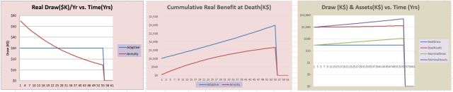
Fig 4 Relax Capital Market Expectations (CME) to: RFR=1.5%, ERP= 4%, Inflation= 2.5%

In Fig 5 below, continuing the evolving scenario where we first increased portfolio risk to 46% stocks and then relaxed the very conservative CME, we next look at the impact of a 50% drop in stock prices after the first plan year. Observations: (1) real draw is unchanged from previous scenario in Fig 4 since there initially available assets were sufficient total expense requirements even after stock allocation was halved in value, (2) real income is maintained at required level to age 120, and (3) Cumulative Real Benefit until death substantially greater with the adaptive approach and gap is not closed until age 120

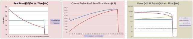
Fig 5 Consider scenario that Stocks Drop=50% after first plan year

And finally, in Fig 6 below, with the more relaxed CME the maximum permissible stock allocation increased from 46% to 56%, but the 10% increase in stock allocation did not result in substantial gains

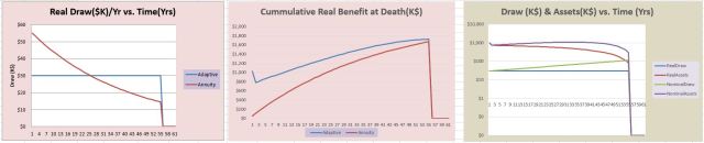
Fig 6 x=56% More relaxed CME allows increase of Stock Allocation to 56%

The tool’s flexibility allows you to explore many other scenarios and outcomes from the complex interaction of the various input factors, like: at what (lower) starting asset level the only option might be the annuity, the power of reducing fixed (and total expenses) to generate a workable plan, the evolving impact of age on plan horizon, average tax impact, the value of pensions (especially when indexed).

Bottom line
The adaptive approach presented in this spreadsheet shows the way to a path to potentially superior outcomes for the complex and often daunting challenge to answer the “How much can I spend in retirement?” question and reduce the fear of running out of money before death. Give the tool a try, I find it useful for my personal planning.

Appendix- Tool/spreadsheet usage- How much can I spend?

(Note: * next to a result indicates a potentially undesirable outcome requiring review

Step 1 Enter required data in ‘green’ sections of spreadsheet in red font cells only (Age, Pension, Assets, Expenses (Fixed, L1, L2) and average Tax-rate)…the derived outputs are also shown in the green areas Plan Horizon (38 years for this 65 year old or age 103) and MaxDraw/yr ($27.6K/yr for portfolio comprised of risk-free assets only) are shown as outputs in green areas
Step 2 The ‘yellow’ area shows the default values of Capital Market Expectations(CME) and default (in cell P18 is ‘50%‘) potential market drop against which we would like to protect the Fixed + L1 discretionary exp’enses in red font cells.
Step 2a The green area of the spreadsheet you can also observe the Maximum/Minimum stock allocations corresponding indicated criteria/objectives. In the only red font cell in the ‘blue’ area you may specify the stock allocation (x%, 0<x<100%) to your retirement portfolio using the guidance provided by the Maximum/Minimum stock allocation in the ‘green’ highlighted black font cells. The selected stock allocation is not necessarily constrained to be less than the smallest Maximum or greater than the largest Minimum, if you can accept the potential consequences of your stock allocation. In this example we could choose as little as 15% (per Criterion 6) instead of  permitted maximum of 46% (per Criterion 1) stock allocation which would still protect Fixed expenses against a 100% stock drop ; ultimately it is an informed judgment call. Once a non-zero (15% in this case) stock allocation was selected MaxDraw/yr(x%Stk)= $30.3K, in the blue section, is higher than $27.6K at 0% stock allocation (below it) and higher the required $30K to cover Total Expenses=Fixed+L1+L2 (above it).
These steps (1, 2, 2a) show you how much you can spend at your selected stock allocation guided by the Maximum and Minimum allocations associated various objectives/constraints. The corresponding Real/Nominal Assets and Draw over the Plan Horizon assuming the unlikely case that the Capital Market Expectations are achieved in each year of the Plan Horizon are shown on the included graph. Of course, this is a very unlikely scenario once stock allocation is non-zero; in practice one would re-run the planning spreadsheet at the start of each year (and after a significant market event, say >20%) with the then current information to generate an acceptable new plan in the context of the new reality. This is what makes this approach adaptive because we correct each year for the new reality.
Step 3 (Optional) An optional step is available if one is interested exploring the impact on Assets/Draw of a significant stock drop at a particular age during the plan horizon. For example, a 50% stock drop in the year after plan start (at age 66) has been specified in the red font cell highlighted in ‘yellow’  in Step 3.
You can explore scenarios of various stock market drops by entering your assumed % drop in the year. For example, if a 50% stock market drop occurs at age 66, the resulting Assets/Draws are shown in the graph.
Step 4 (Optional) Another optional step is to compare the annual real draw and cumulative “spend + bequest” value at various ages of death, up to the plan horizon, comparing the adaptive approach over discussed here with an Annuity (SPIA); the annual Annuity/$1000 is a required additional input in the cell with ‘pink’ highlight written in red font.

 Correction May 1, 2018: The Nominal Assets curve in right-most graphs in Figs 2-6 were corrected in value; the curves in legend associated with those graphs were also previously mislabeled. As the Nominal curves were derived from the Real ones for illustrative purposes only, they had no material impact on the blog post content. Thanks to post reader TW for bringing to my attention.