In a nutshell

How much stock allocation can I have, need to have and should I have in my retirement? Asset allocation considerations in retirement are determined by your personal: goals/objectives, overall financial picture (assets/income and fixed/discretionary expenses), risk tolerance (ability/willingness/need to take risk), required returns, withdrawal rates, taxes and capital market expectations. Management of risks (inflation, market/longevity) in retirement driving/constraining asset allocation are addressed by exploring: minimum/maximum/required stock allocations, trade-offs between stock allocation and expense reduction. Stock allocation in retirement is not some universal age-dependent glide-path that’s at times suggested, but it is a periodically updated allocation based on changing personalized context. A spreadsheet, which I found useful in exploring my own stock allocation space, is provided to help other retirees who might find it useful in exploring their trade-offs. Some arguments, pro/con rebalancing are be touched upon.

The details

(Updated August 10, 2015: A much simpler spreadsheet than discussed below  is available at “Stock allocation in retirement” covering all aspects of this post except the Asset Allocation Implementation towards the end of this post.)

The starting point for any asset allocation discussion must be some of the key elements of the Investment Policy Statement (IPS): goals/objectives, overall financial picture (assets/income and fixed/discretionary expenses), risk tolerance (ability/willingness/need to take risk), required return, withdrawal rate and of course constraints (time horizon, liquidity, tax consideration, leverage, legal, etc); and clearly, with the growing retirement horizons periodically re-vectoring is inevitable due to changes in circumstances over 10-40 years . It is understood that there is no set and forget plan, the future is uncertain and flexibility/adaptability to changing circumstances is essential. The calculation of W-S maximum withdrawal rate and the selection of appropriate stock allocation must be done at least annually to reflect the current circumstances (e.g. assets, expenses, real risk-free rate, inflation, etc.)

What are some of the major goals/objectives of retirees? Retirees’ goals are to (cover expected liabilities in retirement): (1) cover their fixed (basic), discretionary (variable), emergency expenses (which can be allocated as part of liquidity consideration in the asset allocation process), (2) a long-term care (LTC) reserve (to cover the costs incremental to normal living expenses for about 3-5 years of care for one of a couple assuming the other will provide care to the first to need it), and possibly (3) a discretionary (except in cases when a family member is disabled which might make it necessary) bequest allocation (to family, charity, etc) which can also act as a safety valve to help deal with unbudgeted expenses or lower than assumed returns.

For incremental long-term care reserve a starting ‘plug number’ might be in the range of $150K-$200K. For bequests, assets in excess of those needed to meet annual expenses, long-term care reserve and absolutely essential bequests (e.g. funds needed for the care a disabled family member) would be potentially available for additional discretionary or desired bequest reserves. We will dispense with the LTC/bequest goals since the W-S withdrawal rate (based on very conservative planning horizon) is sufficiently conservative in most situations; should one wish to include these, the simplest way would be by reducing the assets available for income generation accordingly) . Speaking of assets available for income generation, your home that you’re living in should not be included into the assets unless you are explicitly planning to sell it to generate income.

Assets, income and expenses

Any lifetime income streams (e.g. pensions) will be used to offset fixed (and discretionary once fixed is covered) expenses. Available Assets can then be used to cover the expenses not covered by lifetime income sources. You will need to gather up information associated with all assets (e.g. bank and investment accounts, and real estate available for sale).  The process is inherently iterative; if assets are far in excess of income needs/desires then there is opportunity to re-balance discretionary expenses vs. bequests; if assets are insufficient, even after introducing an acceptable level of risk, then it is necessary to re-examine and perhaps reduce proposed view of expenses before other heroic efforts are considered.

To determine retirement income needs, we will not be using arbitrary/inappropriate preretirement income replacement percentages like 50% or 70-80% or 100% of income or working backwards from a (so called) “sustainable” withdrawal rates from assets (e.g. a rigid 3% or 4% of initial assets, then annually adjusted for inflation). Instead the retirement expenses should be calculated based on tracking actual expenditures in retirement, or for pre-retirees on actual pre-retirement expenses modified for additions (e.g. more travel) or deletions (e.g. no retirement savings).

The implementation proposed here starts with identification of after-tax expenses which are then grossed up for taxes (to before-tax expenses) and then reduced for pensions (lifetime income streams such as OAS/CPP or Social Security and any applicable employment related pension). Expenses are separated into: fixed (such food shelter, utilities, insurance, type expenses which must be covered), and discretionary expenses which are more lifestyle related; in fact discretionary expenses can be divided into Level 1 (L1- refers to discretionary expenses which might take time to eliminate, such as costs associated with a 2^nd home) and Level 2 (L2- refers to discretionary expenses which can be eliminated almost immediately, such as travel/entertainment/restaurants/gifts).

The Fig. 1 portion of the spreadsheet will be used later to gather most of the required inputs necessary to start discussing asset allocation. NOTE: If you are ready to try it now…In Microsoft Excel 2007 the link opens in Excel Online. Then click on ‘Edit Workbook’ on top and select from dropdown menu ‘Edit in Excel Online’   OR  on the top far right side click on the 3-dots and from dropdown menu select “download a copy” . You are now ready to go!  Also note, that you may click on any of the Illustrations below to enlarge them and make them more readable; when done with it, just click on “Back” button of your browser to continue reading the blog post.  (A simpler version of this spreadsheet is now available here.) Remember that we’ll be building on the W-S approach to calculate maximum permissible withdrawals using a risk-free portfolio (i.e. excludes risky assets in general, and stocks in particular), as shown below:

Note that all numbers shown in red with light blue background are required inputs, while all numbers shown in black with light blue background are legitimate defaults (at the time of writing this post) but may be changed by you. However all other numbers without the light blue background are calculated and thus not permitted to be changed; should it have been changed accidentally you can restore default spreadsheet by reloading again.

What people want from asset allocation?

When speaking of asset allocation, we have typically moved beyond a risk-free portfolio and we’ll be allocating some of the assets to risky investments in the expectation of receiving an increased return, i.e. a premium for taking on the risk. In a 2009 blog post Asset Allocation II I discuss different asset allocation perspectives (in addition to definition of what constitutes an asset class and what asset allocation is and why it is important for investors). There I quote Richard Ennis’s “Parsimonious Asset Allocation” article from the CFA Institute’s Financial Analysts Journal (a great asset allocation read by the way) which dispenses with the diversification arguments (uncorrelated assets), some of the ‘hows’ of asset allocation, and targets directly the ‘whats’ or results that investors really want from asset allocation, and he identifies three things: (1) downside protection ( using “nominal- and real-pay U.S. Treasury securities of varying maturities”), (2) capture as much equity (risk) premium as possible without compromising downside protection (using “a global stock index fund”), and (3) some additional excess return (alpha) should the investor or her adviser be able to identify/exploit some market inefficiency or liquidity premiums . In order to simplify our discussion and due to the challenges associated with such ‘alpha’ opportunities, we will focus only on the first two of these categories, “downside protection” and capturing “equity risk premium”, and how these can be used to build on top of the Waring-Siegel (abbreviated as W-S) approach to achieve retirement goals/objectives and manage the risks in retirement.

Risk Tolerance

Since we are contemplating additional risk (stocks in this case) in our portfolio, we’ll first review (and understand) what ‘risk tolerance’ is about. Risk Tolerance’ is a measure of the combination of ‘willingness’ and ‘ability’ to take on risk.

‘Willingness’ to take risk is a qualitative measure for one’s inclination to be exposed to risk (or more precisely the unknown outcomes). Some try to assess one’s willingness to take risk by a series of hypothetical questions about one’s willingness to accept some percent of portfolio losses in the future. But better qualitative indicators might be how one actually behaved in the past. So an indicator of low willingness to take risk might be: historical and/or current asset allocation only or primarily into CDs/GICs and/or government bonds, difficulty sleeping at night after stock market drops 10-15% and  if significant portion of your portfolio was allocated to stocks and you sold much of your stock allocation during the 2008-2009 market drop. On the other hand if you historically/currently feel comfortable with a significant stock allocation in your portfolio, you don’t lose sleep when the market drops 10-15% because you are invested for the long-run, and rather than selling on the way down in 2008-2009 market rout you rebalanced your portfolio to your target asset allocation and took advantage of opportunity to buy cheap assets (stocks) and sell appreciated assets (bonds). Nobody likes to lose money, but some people can be quickly demoralized into selling assets which are dropping or have dropped in price even if the assets were intended to meet long-term expenses far into the future even though they have the necessary liquidity to meet their short and intermediate term needs. So ‘willingness’ is a qualitative psychological measure of our predisposition to risk.

‘Ability’ to take risk is a quantitative measure of, for example, one’s capability to meet fixed and even discretionary expenses even after (say) a 50% (or even larger) drop in the value of the stock allocation of one’s portfolio. Such measures will help determine maximum stock allocation and implicitly the complementary minimum low/no- risk fixed income asset allocation. The specific implementation of the fixed income portion of the portfolio influences the extent of readily available liquidity to meet needed near-term or emergency expenses over sufficient period (2-5 years) so as not to be forced to sell significantly depreciated assets during a sudden substantial market drop or in a sustained bear market. This can be achieved combination of cash, GIC/CD ladder or even short-term investment grade bond ETFs. (This is not very tough decision nowadays given that there is little reward for locking funds away for >5 years or accepting term risk on bonds.)

When willingness and ability to take on risk are both low or are both high then, the combined effect of these, called risk tolerance is clearly low and high respectively. The more difficult situation is when there is a tension between willingness and ability; i.e. willingness is low but ability to take risk is high, or vice-versa i.e. willingness is high but ability is low. Factoring in ‘need’ to take risk (as in the former case) or a redefinition (up or more likely down in the latter case) of goals/objectives (fixed and discretionary expenses, bequests, etc) specified in the IPS may be helpful to resolve the deadlock.

‘Need ‘to take risk is driven, as noted by Ennis above, by the desire to “capture as much equity premium as possible without compromising downside protection “.  The proportion of the portfolio allocated to stock determines how much of the potential equity risk premium can be expected to be captured, but at the same time determines the downside portfolio risk as well.  So the need to take risk is guided by the required portfolio return to achieve goals and objectives.

So we can assess “willingness” by looking at our current portfolio allocation to risky assets and how we behaved during past crises. Is our “willingness to take risk” low or high?

“Ability to take risk” and “need to take risk” will be discussed later when we look at stock allocation quantitatively; the former (in concert with ‘willingness’) will cap the maximum stock allocation and the latter will drive minimum allocation. However, on the subject of ‘willingness’ (the emotional side of risk taking) you also need to consider Dan Ariely’s take on the subject in the WSJ’s “It’s risky to rely on retirement questionnaires” in which he suggests that it is best to “Figure out what your life might look like with various investment approaches, figure out which trade-offs you are (and are not) willing to make, and plan your investments accordingly. Meanwhile, you can deal with your fear of risk directly. Learn yoga, meditate, take some medication, avoid looking at your portfolio more than twice a year. Do whatever you need to deal with your emotions, but make sure that it doesn’t interfere with the way you decide to invest.”

Risks in retirement

The three major risks in retirement are: longevity risk, market risk and inflation risk. Longevity risk is the risk of outliving one’s assets i.e. running out of money before dying because one did not assume a sufficiently conservative planning horizon, e.g. what not to do is just planning to life expectancy (from current age) which 50% of the population outlives by definition. Market risk is the risk that an unexpected market crash (e.g. 2008-2009) in general or a sustained bear market will result in a one large or sequence of smaller negative returns which then compounded by annual withdrawals will grind assets down to exhaustion well before one dies. Inflation risk, the silent killer, will gradually corrode the purchasing power of constant nominal annual withdrawals or income streams (annuities and unindexed corporate pensions), so that even a 2.0% annual inflation rate will reduce the purchasing power of $1 will half (54¢) over a 30 year retirement.

How to tackle these retirement risks?

Consider the three approaches for the three risks:

1. For longevity risk, consider Waring & Siegel’s dynamic spending rule based on ARVA or Annually Recalculated Virtual Annuity”. ARVA effectively recalculates each year (without actually buying the annuity) the income that you would get if you could buy a fairly priced level payment fixed term real annuity based on current: (1) real risk-free rates, (2) a conservative estimate of how long you’ll need the income (the average of lifespan (120) and life expectancy), and (3) the available assets. They discuss this approach in their paper entitled “The only spending rule article you’ll ever need” which I reviewed recently in this blog post. This is how the maximum annual permitted withdrawal rate from a risk-free portfolio is determined annually to insure that one doesn’t run out of money while still alive. (Some consider longevity risk as the risk of taking excessively high withdrawals which lead to running out of money before death.)
2. Market risk results when instead of a risk-free portfolio, many retirees accept some risk in their portfolio by allocating part of their assets to stocks; increasing the portfolio risk in this manner (but still consistent with one’s risk tolerance) gives one the opportunity to further increase annual income and potentially preserve (or even enhance) much of the starting value of the portfolio at least in nominal (if not real) terms. With a risky portfolio, using Waring and Siegel’s dynamic spending rule, you effectively would be recalculating the fixed term virtual annuity each year based on the changing value of your risky portfolio (which might be higher or lower than previous year depending of the combined effect of the withdrawal and the stock market performance) and the new somewhat shorter annuity term each year. One particular subset of ‘market risk’ is the ‘sequence—returns’ risk’, whereby the market doesn’t drop all at once 30-50% but it get’s ground down 15-20% per year for 3-years in row for a total loss of perhaps close to 50% further aggravated by failure to rein in spending to an acceptable level. With a risky portfolio you must be able to live your life with some spending flexibility/adaptability (e.g. if necessary trimming back on some of the desired discretionary spending). Waring & Siegel explain that “one’s risk tolerance for the investment portfolio is equivalently one’s risk tolerance for spending volatility.” But how do we determine what would be an acceptable asset allocation for a portfolio composed of two asset classes:  fixed income and stocks. We might try to find two bookends for stock allocation. One bookend might be determined looking at what’s the maximum permissible stock allocation so that: (1) a 100% stock loss would still leave sufficient assets to cover our fixed expenses (and perhaps even maintain some level of flexibility), or (2)  a 50% (or some other percent)  stock loss would still allow coverage of fixed plus more difficult to shed Level 1 (L1) discretionary expenses, or  (3) using Charles Ellis’s  recommendation that any assets not needed to cover the next 10 years expenses can be allocated to stocks (risky assets)
3. For inflation risk, Waring and Siegel’s paper demonstrates that annually repeating their virtual fixed (though decreasing) term annuitization even for a constant real rate of return (of 0.6% at the time of writing their paper but since dropped to about 0.2% now) , the resulting nominal income stream offers some level of inflation protection well into one’s “eleventh decade”, primarily due to increased maximum permissible draw driven by the decreasing term of the fixed virtual annuity each year as one ages (i.e. it has some built-in inflation protection on the nominal distributed income, which by the way is composed by a combination of the real interest on remaining assets and the return of one’s own capital). So one bookend, the maximum, was the maximum was discussed in the ’market risk’ section above.  The other bookend might be the minimum stock allocation needed to increase the (risky) expected real return sufficiently: (1) to make expected maximum draw rate equal required total expense draw rate as a percent of assets (of course when the actual return is lower than the expected return, we’ll have to absorb some of the shortfall by reducing discretionary spending which acts as shock absorber), or (2) to generate an expected return to restore nominal assets after drawing the Total expense from the portfolio, or (3) to restore real assets after Total expense draw.

In Fig. 2 we assume ‘Real risk-free return’=0.2%, ‘Inflation’=2% and an Equity Risk Premium = 4%; ’stock ‘volatility’ or ‘standard deviation’ (SD)=16%. Therefore ‘nominal risk-free return’= 2.2% (0.2%+2.0%) while nominal stock return= 6.2% (2.2%+4%).

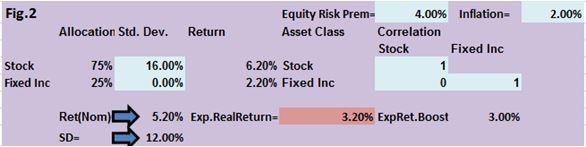
By just plugging in the appropriate numbers in the Fig. 1 where stock allocation is input, then in Fig. 2 portion on the spreadsheet one readily can see that a 25% stock allocation would boost expected return by 1%/ year (from real 0.2% to real 1.2%), while a 50% stock allocation would boost expected return by 2% (to real 2.2%) so at least in nominal terms it might be expected overcome on the average the 2% inflationary headwind over this retiree couple’s life; all this is assuming that they can bear the income volatility accompanying the level of stock allocation. Waring and Siegel point out that the standard deviation of the income would be the same as that of the portfolio returns.

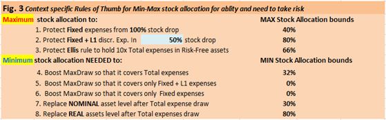
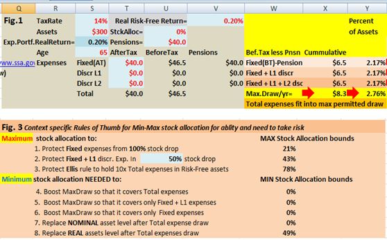
So the stock allocation bookends might, for example, be determined by a maximum which protects the asset coverage of Fixed and/or ‘Fixed + Level1’ discretionary expenses following a 100% and/or 50% respectively (or you pick other maximum market drops scenarios) or the typically less constraining Ellis rule-of-thumb which suggests keeping 10 years of income requirement in low risk fixed income assets and a minimum which will boost expected average return so that maximum permissible draw is raised to the level of total expenses, or provide some mitigation of the corrosive effects of inflation subject to willingness/ability to deal with an occasional reduction of the desired discretionary expenses. These bounds are listed in Fig. 3 portion of the spreadsheet; examining these 8 bounds listed, 3-maximums and 5- minimums, might together with our willingness to take risk, will help guide us to our appropriate stock allocation. For example

Asset allocation helping manage risk in retirement

So asset allocation plays a significant role in dealing with all three retirement risks: longevity risk, market risk and inflation risk. But it won’t work for everyone; those whose willingness and ability to bear risk are very low, specifically those whose fixed expenses cannot be reduced proactively/voluntarily to a level to where some portfolio risk can be assumed by transforming some fixed into discretionary expenses to create some shock absorbing capability in the portfolio, might have to even accept (partial) annuitization which will likely lead to a involuntary but gradual/continuous reduction of the buying power of a nominal annuity, with inflation eroding coverage for ‘fixed’ expenses. Finding the balance between need/desire to spend and asset protection for the future, and having the ability to handle the income volatility when markets drop (even precipitously), to have sufficient remaining assets to fight another day and then benefit from the historical/eventual market rebound, makes asset allocation an essential tool to meeting retirees’ goals/objectives articulated in their IPS.

Maximum stock allocation To bookend maximum stock allocation we could use: (1) maximum tolerable loss at 50% (which is changeable to some other level e.g. 40% or 75%) of stock drop which will still leave sufficient assets to deliver the required income for Fixed plus L! discretionary expenses, or (2) maximum tolerable loss at 100% stock drop while protecting Fixed expense coverage, or (3) Charles Ellis’s recommendation of protecting 10 years of (e.g. Fixed or Fixed+L1 discretionary or Total) expenses with safe fixed income assets and using the remaining assets available for stock allocation. (See Fig. 3 for the three values of these maximums for a specific retirement circumstance.)

Minimum stock allocation To get some handle on a minimum stock allocation (assuming 4% equity risk premium, i.e. the expected real equity returns are real risk-free return plus 4%) let’s explore the return required to replace the withdrawal (rate), in order to preserve the nominal value of the assets (similarly we could explore the return required to preserve the real value of the assets). So disregarding return and income volatility for the moment, then assuming 0.2% real return with an inflation of 2%, then the risk-free or 0% stock allocation (entered in Fig.1) would deliver a nominal return of 2.2%; similarly nominal 3.2% and 4.2% return would be delivered at 25% and 50% stock allocations, respectively as shown in Fig.2 for an “Equity Risk premium”=4.0%. Therefore, when we draw 3.4% of assets then to just maintain on the average the nominal level of assets we need to earn 3.4% return which in this case would imply increasing the portfolio risk to a minimum of 30% allocation to stocks. The formula for Minimum Stock Allocation = (Required Return-RiskFree Return) / (Stock Return-RiskFree Return). If we would like to compensate also for inflation then the minimum stock allocation would have to also compensate for the 2% assumed inflation i.e. for a total return of 5.4%  (3.4% draw + 2% inflation) requiring 80% stock allocation.

Trade-offs in managing risk in retirement between  fixed expense reduction and stock allocation With these assumptions (real fixed income return essentially zero (0.2%), 16% standard deviation for stocks and zero for fixed income assuming relatively short maturity safe fixed income investments, equity risk premium 4%, and zero correlation between fixed income and stocks) to increase return rate by 1% we must add 25% additional stock allocation which brings with it increased volatility of 4.0%; but note that if equity risk premium is only 3%  (rather than 4%) then we’d only get 0.75% expected average return improvement for each additional 25% allocation to stocks. And as indicated above, maximum stock allocation is constrained by downside protection necessary to protect income coverage for fixed expenses. Looking at how maximum withdrawal rate changes as real return changes under the Waring-Siegel strategy, each 1% increase in real (risk-free) rate translates into about 0.5% of increased maximum withdrawal rate. So each incremental 25% stock allocation delivers only 0.5% of incremental maximum withdrawal rate. So in reality the most effective control mechanism for retirees to combat the major risks in retirement (longevity/market/inflation) is expense minimization in general and fixed expense minimization in particular, in order to prevent excessive withdrawals from reducing assets to a point of no return.

Age dependent stock allocation? As to the debate about the traditional view that you should be decreasing your stock allocation as you age (e.g. allocating (100-age) or (110-age) percent to stocks vs. just using an age independent balanced portfolio (e.g. 60% stocks and 40% fixed income) or even the more radical recent proposal to actually increase the proportion of stock with age, my view has not changed in years. The stock allocation is not determined exclusively by age, but it is determined by the individual’s or couple’s circumstances, the most important of which is risk tolerance, as discussed above. But having said that age not the governing factor to stock allocation, it can come into play especially as one examines near end-of-life scenarios due to investment horizon considerations. When someone or some couple is in their 90s, then using the Ellis rule-of-thumb of allocating 10 years’ worth of expenses to fixed income, and assuming annual costs (depending on the level of support that might be required) ranging from $60K-$120K+/year, so a corresponding fixed income allocation might be $600K-$1.2M+ which would effectively drive most retirees in their 90s into 100% fixed income allocation. (The W-S strategy for 90 year old couple (using the very conservative female as a proxy for joint mortality) allows 6% and 7.2% maximum draws at ages 90 (17 year planning horizon) and 95 (14 year planning horizon) respectively; for male mortality the corresponding draw rates are 8.4% (14 years) and 11.3% (11 years) respectively. As you’ll note the W-S assumed planning horizons are quite conservative, so if necessary there may be some opportunity to relax these. ) But driving retirees to a higher stock allocation in general is the need to combat inflation; this however is less compelling of an issue for retirees in their 90s typically since the corrosive effect of inflation is less damaging over a shorter 10-15 year horizon vs. a potentially 30-40 year horizon for a 65 year old couple. Therefore a higher or even an exclusively fixed income asset allocation, with its lower associated market risk, would be acceptable. Of course, if assets in the 90s are still well in excess of  $2M+ in this example, then correspondingly higher ability to bear risk would still permit a substantial stock allocation, but willingness/desire and ability to manage investments, especially for DIY investors, would still limit exposure to risk unless driven by substantial bequest motives.

Scenarios

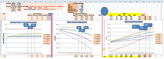
Starting point for withdrawals is expenses (Fixed +discretionary L1 and L2), i.e. how much do I need/want rather than take the maximum allowable percent under the Waring-Siegel approach. As a reference the current annuity rate available for a 65 year old couple in Canada is about nominal 5%/year; of course this requires that the capital  be irreversibly handed over to an insurance company, i.e. loss of control over the capital. (Aside: For 65 year old Nortel retirees who are contemplating a cash value vs. annuity decision, if the cash value offered (e.g. $5K/yr annuity but only $80K cash value) implies a much higher annuity rate (5/80=6.25%) than available in annuity markets (currently5%), that’s an indication of significantly low-balled cash value rather than a great annuity rate. Still this may drive you to take the annuity (even though you might prefer the cash value at the market rates) so you have to be careful in the decision process. Also Canadian pensioners need to keep in mind that annuity payments are comprised of interest (on government of Canada bonds), mortality credits (but typically based on 60-70^th rather than median percentile mortality assumption plus a return of pensioners’ own capital. Annuities are insurance, not an investment and they essentially trade off longevity for inflation risk.)

We are now ready to look at some examples; the spreadsheet is accessible at the following link. NOTE: If you are ready to try it now…In Microsoft Excel 2007 the link opens in Excel Online. Then click on ‘Edit Workbook’ on top and select from dropdown menu ‘Edit in Excel Online’  OR on the top far right side click on the 3-dots and from dropdown menu select “download a copy” . You are now ready to go!  (A simpler version of this spreadsheet is now available here.) The most important moving parts influencing the analysis are: assets, expenses (fixed and discretionary), and sources of lifetime income (pension income). Other important factors are age (an important element driving planning horizon), tax rate and real risk-free rate available in the market.

Scenario 1A

All we need to get started are the following inputs shown in red in Fig. 1 of the spreadsheet:

Age= 65 year old couple

Assets ($K) = 1000

Income ($K)(lifetime)/yr (e.g. pensions, annuities, etc) = 30

“Fixed” Expenses ($K)  (expenses that must be covered involve food, shelter, medical, insurance…) = 40

Discretionary L1 Expenses ($K) (Level 1 discretionary refer to expenses which may take time to reduce/eliminate e.g. expenses associated with a 2^nd home) = 0

Discretionary L2 Expenses ($K)  (Level 2 discretionary expenses refer to expenses which can be shed quickly if necessary, e.g. travel, entertainment, restaurants…)= 15

Total Expenses (Calculated)= Fixed + Discretionary L1 + Discretionary L2 =40+0+15=55)

Tax Rate (average)= 14%

Real Risk-Free rate (currently)= 0.2%

(Inflation=2%. Equity Risk Premium = 4%. Both are changeable)

Stock Allocation= 0% (0% starting default as per W-S risk-free portfolio but final allocation is TBD based on Minimum and Maximum bounds in current context)

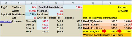
The left hand portion of Fig. 1 in the spreadsheet summarizes the input and gives a quick assessment of how close we are from meeting our goals and objectives:

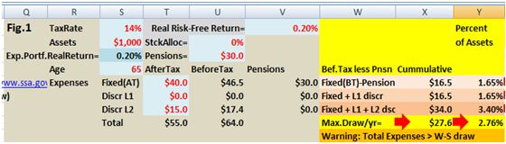
Here with a risk-free portfolio the significant assets and pensions appear inadequate to meet our goals/objectives. Note that the Total expenses (fixed and discretionary) after gross up for taxes and offset by pensions amount to 34.0K which is 3.4% of assets but above the maximum withdrawal rate of 2.76%.

Our objective is to adjust expenses and/or stock allocation to a level where for the next year the Total expenses (Fixed+ L1+ L2) are less than the MaxDraw permitted. As you can see above, that is not the case as noted in the note highlighted in orange Warning: Total Expenses > W-S draw

Scenario 1B

One option would be to try to reduce discretionary expenses so they fit within the maximum envelope. Reducing discretionary L2 expenses from $15K to $9K gets us to a Total (Fixed+L1+L2) withdrawal rate of 2.7% which is below the maximum withdrawal rate of 2.76%.

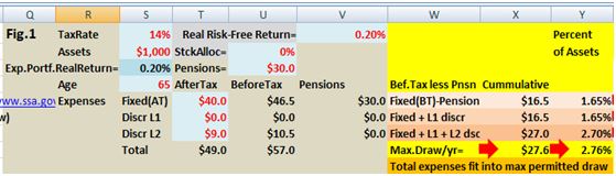
Our objective was to adjust expenses and/or stock allocation to a level where for the next year the Total expenses (Fixed+ L1+ L2) are less than the MaxDraw permitted has been achieved by reducing L2 discretionary expenses from $15K to $9K. The note highlighted in orange above now indicates that expenses fit as they are at a level below MaxDraw. Note the message highlighted in orange now indicates Total expenses fit into max permitted draw

 

Scenario 1C

Or, we could return to Scenario 1A and leave L2 expenses at $15K and let’s examine Fig. 3 which looks at some boundary conditions for adding some stocks to the portfolio.

Rule-of-Thumb #4 (RoT #4) suggests that a minimum of 32% stock is required, while Rules-of-Thumb 1, 2 and 3 cap maximum stock allocation at 40%, 80% and 66% respectively (all above 32% minimum); depending how much we value each of these criteria we might consider a stock allocation ranging from 32% to 60% (e.g. if RoT scenario of 100% stock drop is considered highly unlikely) ; 32% and 60% stock allocation, when plugged into Fig. 1 sequentially, deliver real returns of 1.48% and 2.6% respectively (shown in Fig. 2)(though not risk-free). Note in Fig.1 Expected Real Return is automatically updated with each stock allocation change.

Using 32% which boosts expected real return from 0.2% to 1.48%, and the MaxDraw to 3.44%, thus expected to cover Total expenses as predicted. Of course we are now using risky assets and the 1.48% might be expected but is not guaranteed; should it come in lower, then expected assets will be lower and we will have to reduce future discretionary expenses.

Scenario 1D

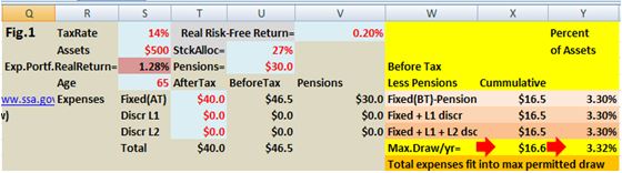
Suppose this couple just inherited winter home from their parents, and they have determined that it would cost them annually additional $10K (L1 expenses) to keep it and become snowbirds; they are prepared to reduce their L2 discretionary expenses from $15K to 10K. So we update the data in Scenario 1A by changing Discr L1 expenses from $0K to $10K  (L1 type expenses differ from L2 in that they are more difficult to shed) and reduce Discr L2 expenses from $15K to $10K. (Remember to reset StckAlloc=0%)

Then the new Fig. 1 shows adjusted L1=$10K and L2=$10K discretionary expenses, the result indicates Total Expenses (Fixed+L1+L2)=3.98% > MaxDraw=2.76%

However Fig. 3 on Min/max recommendations becomes

Now we need to choose an acceptable stock allocation based on how much we value each of these criteria. If we strongly desire to keep the seasonal home (L1=$10K) and the L2 discretionary spending at $10K, then we may be prepared set higher stock allocation (start at 61% guesstimate in Rule-of-Thumb #4 and adjust the stock allocation gradually downward until we reach the lowest percent stock allocation which results in Total expenses (Fixed+L1+l2) < MaxDraw) then 56% the minimum required to boost MaxDraw to 4.00% > Total expenses=3.98%, so that

Scenario 1E

Suppose that we wanted to tackle Scenario 1B except the available assets are $500K instead of $1000K.

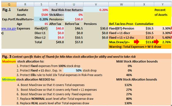
This picture looks somewhat grim, since MaxDraw at $13.8Fig. 1, which reduces Total expenses and increases RoT #3 maximum from 46% to 67% stock allocation. Also looking at some opportunities that we can glean from the Fig. 3 Min-Max analysis, we observe that the least stringent maximum is RoT #3 (at 46% or 67%) eliminates all minimum RoTs but RoT #6 of 27%. But any non-zero stock allocation would violate RoTs #1 and #2 which in this case indicate that any non-stock allocation would put at risk even more of the Fixed expenses of $16.5K; in fact, even with Stock Allocation= 0%, the Max.Draw permitted with the W-S process would be 2.76% or $13.8K which is $2.7K below the Fixed expenses.

But if we are prepared to forgo the protection of the Fixed expenses from say a 50% (or more) stock drop, the 27% stock allocation would raise expected real return sufficiently to increase MaxDraw to 3.32% (driven by the average return expected from the stock allocation to be a real 1.28% or nominal 3.28%) and could be expected to cover the fixed expenses.

But if we insist on being able to absorb with 50% stock drop without affecting coverage of Fixed expenses, then we’ll need to either: (1)  start reducing Fixed expenses (by $2.5K or 6.25% to $37.5K we could achieve income stream using W-S approach with a risk-free portfolio yielding just 0.2% real, or (2) consider self-annuitizing for a 20 year fixed term (to age 85) $324K at 0.2% real risk-free rate to generate $16.5K/yr, and simultaneously buying at age 65 a $25K/yr longevity insurance with income starting at age 85 which costs for a male $50K and for a couple $87K pricing from Forbes article (available only to American retirees); at 2% inflation the $16.5K/yr income in 20 years become $25K) or (3) consider perhaps partial annuitization; it all depends on our risk tolerance.

As an aside instead of using the W-S approach, with the 27% stock allocation and the corresponding expected 3.30% annual draw, a Monte Carlo simulation using the Ceiling/Floor approach with setting the draw Floor=0% (meaning that we don’t allow changes in return to reduce draw below the 3.3% floor (or $16.5K). Here we end up we a less than 5% probability of running out of assets over 40 years (i.e. age 105 for 65 year olds) and a 50% probability of still having Assets >$365k, as shown below

This suggests that unless we have some very unpleasant sequence of returns problems, we might even consider proceeding with the 27% stock allocation.

Another approach to resolving this impasse is to remember that there if we could find a way to relax, just a little bit, our Fixed expenses (which so far we assumed that we can’t encroach on) then we may come up if a far superior solution. So instead of increasing risk, if we could live with Fixed expenses=37.5K, we would be able to leave Stock Allocation at 0% and still keep expenses at 2.72%

Scenario 1F

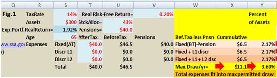
Continuing from Example 1E but consider that we annuitize $200K yielding nominal $10K additional lifetime income per year. A 65 year old couple can get a joint annuity at a 5% rate (in Canada). This would reduce assets from $500K to $300K and increase annual pension by nominal $10K from $30K to $40K

This moves Total expenses (2.17%) < MaxDraw (2.76%) and would allow up to 43% stock allocation and still protect coverage Fixed expenses from a 50% drop in stock prices, transforming the scenario to this

I personally found this spreadsheet a useful tool to explore various scenarios given my circumstances. I hope that it might also be useful to other retirees to explore their asset allocation space in their search for a solution that they can live with in retirement. (Comments welcome whether you agree or not.)

Asset Allocation implementation

In Fig. 1 of the Annuity/Pension vs. Lump-Sum- Part 3: Quantitative considerations we discussed some Capital Market Expectations for various asset allocation based  on Vanguard’s crystal ball, but considerably (about 25%) lower return expectations have been used here to reflect the generally lowered return expectations since then; standard deviation used was left at similar order of magnitude, at 16% (compared about 17.5%)

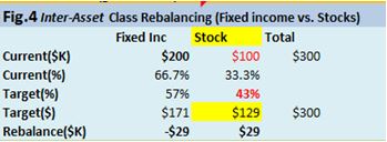
In this post I have used only two asset classes: fixed income (implemented with essentially risk free GICs/CDs or high quality short term bond funds in home currency) and stocks (US CD rates are slightly lower than those available in Canada, but not by much.) Figs. 4-8 in this spreadsheet consider various aspects of implementation of such an approach: starting with your existing assets already specified in Fig. 1 of the spreadsheet using the last Scenario 1F with Assets=$300K and Stock Allocation= 43%, the current Stock Allocation in dollars ($), the target Stock Allocation in percent (%) from the analysis such as discussed in the earlier portion of this post, you get the fixed income and stock allocation changes (in dollars) that you’d have to make to achieve your target allocation. We then continue with Figs. 5-8 to further sub-allocate the stock portion of the portfolio using different approaches and ETFs to implement the desired portfolio.

Once we have determined the fixed and stock allocations of our current portfolio, then using our target portfolio’s percent of stock allocation, we can then calculate the changes required to our current portfolio to align it with this new target. Fig. 4, where this is referred to as “inter-asset class” (i.e. between stocks and fixed income) rebalancing, shows how this calculation is done. You just need the required inputs, shown in red. (Note that total portfolio size is taken from the “Assets” specified in the top left-hand corner of the spreadsheet and one needs to only enter the dollars allocated to the  fixed income portion of the portfolio, and the target stock allocation; everything else is calculated automatically.

Figs. 5-8 show some of the possible “intra-asset class” allocation approaches that Canadian and American investor might take; the overall asset class referred to here is stocks, which may be further broken up into (sub-) allocations to US, Canadian, international, and emerging markets with some of the possible approaches that one might take.

Fig. 5 shows a simple (two-ETF) implementation of the stock portion of the portfolio for an American investor. This is composed of two Vanguard (US based) ETFs: VTI (Total US stock market) and VEU (Vanguards All-world stock market ex-US, i.e. the Rest-of-the-World which include developed and emerging markets). The only inputs required  here are the dollars currently allocated to home (US) based stocks and the target percent of US stocks out of the total tock allocation (50% was chosen here)

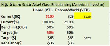
Fig.6 shows a simple (three ETF) implementation of the stock portion of the portfolio for a Canadian investor. Here the implementation is done Vanguard (Canada based) ETFs with stock allocation is equally divided into three markets: Canadian (VCE), US (VUS CAD-hedged or VUN un-hedged) and International (VEF CAD-hedged or VDU un-hedged, based on FTSE developed ex-North America index. i.e. no emerging markets allocation). Note that a Canadian might choose CAD-hedged or un-hedged versions of the US/International allocations. A Canadian retiree who is a snowbird spending significant time in the US, might choose the Vanguard Canada based un-hedged version of the US market ETF VUN or even the Vanguard US based USD implemented VTI ETF.

Fig.7 shows my personal stock sub-allocation with Canada, US, EAFE (developed markets ex-North America) and Emerging Markets with target allocations of 25%, 30%, 25% and 20% (which is overweighed, for better or worse,  in EM stocks due to valuation and GDP growth considerations.)

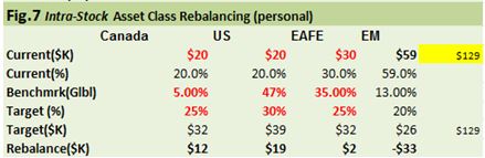
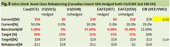
Fig. 8 for Canadian investors, builds upon Fig. 6 and Fig. 7 and further diversifies the stock allocation by splitting each of the US and International stock allocations (50:50) into CAD-hedged and un-hedged portions as shown below and did not overweigh the emerging market allocation.

Rebalancing

The mechanics of rebalancing have been built into Figs. 4-8 of the spreadsheet. There is a no absolute consensus about the value and purpose as well as timing of rebalancing; i.e. is it worth the trouble? As discussed there are two kinds of rebalancing considered here: the” inter-asset class” which to a large extent is the risk control mechanism, i.e. can be used to control our downside risk. The “intra-asset class” rebalancing may be considered as an approach to periodically drive us to sell some relatively overvalued stocks (regions) and buy relatively cheaper stocks (regions). There are also some who argue that buy-and-hold is the right approach (i.e. let the winners run or momentum approach) and do rebalancing only using new money (income or interest/dividends). The whole rebalancing topic is complex as it also involves tax considerations, so I would be inclined to say is that it should be done opportunistically except when downside risk considerations require action.

Bottom line

So there is no generally applicable answer to retirees’ stock allocation. The decision on the most appropriate stock allocation is very personal. The drivers of what’s appropriate asset allocation include many of the key inputs to an Investment Policy Statement such as: goals/objectives, overall financial picture (assets/income and fixed/discretionary expenses), risk tolerance (ability/willingness/need to take risk), required returns, withdrawal rates, taxes and capital market expectations. Management of risks (inflation/market/longevity) in retirement driving/constraining asset allocation are addressed by exploring: minimum/maximum/required stock allocations, trade-offs between stock allocation and expense reduction.

This tool/spreadsheet was useful for my exploration of various approaches given my circumstances. (A simpler version of this spreadsheet is now available here.)  I hope that it might also be useful to other retirees to explore their asset allocation space in their search for a solution that they can live with in retirement. As usual, any comments/suggestions/views are always appreciated.