In a nutshell

In this blog post (Part 3 in the series), in the context of a specific example for a 67 year old couple, we explore quantitative considerations toward the annuity/pension vs. lump-sum decision, such as: (1) fixed and discretionary expenses, (2) capital market expectations, (3) how/when/if to annuitize, (4) understanding the value delivered by an annuity as measured by the implied IRR (Internal Rate of Return) and NPV (Net Present Value) as a function of actual longevity, (5) alternatives to annuitization: self-annuitization and systematic withdrawal strategies using NPV to compare decumulation strategies, (6) bracketing the portfolio risk/asset-allocation (and return) between minimum return requirement (or minimum risk/stock-allocation required) and maximum portfolio return (risk/stock-allocation) by stress testing portfolio with a 50% stock market drop and (7) what are triggers to annuitization.

This five part series on Annuity/Pension vs. Lump-Sum is composed of: Annuity/Pension vs. Lump-Sum- Part 1: Making the right decision for you which explores risks in retirement,  Annuity/Pension vs. Lump-Sum- Part 2: Drivers to and away from annuitization  focused on qualitative considerations toward the annuity/pension vs. lump-sum decision,  Annuity/Pension vs. Lump-Sum- Part 3: Quantitative considerations focused on quantitative considerations in the decision,  Annuity/Pension vs. Lump-Sum- Part 4: Monte Carlo simulation to explore retirement income trade-offs with and without annuitization where Monte Carlo simulation is used to explore the range potential outcomes given assumed Capital Market Expectations, (risk tolerance and corresponding) Asset Allocation, in the context of personal circumstances (Age, Assets, Expenses, Other Lifetime Income sources and the resulting required withdrawal rate) and compare these with annuitization. Then in order to help see the entire picture, in the 5^th and final part of this series  Annuity/Pension vs. Lump-sum- Part 5: Putting it all together  I use the case of an 85 year old single male with a life expectancy (i.e. 50^th percentile) of the order of 5 years and a 90^th percentile life expectancy of about 11 years, instead of the mostly used 67 year old couple who needed to finance a potentially 30 year long retirement.

 

Disclosure and warning

Note that none of what follows should be construed as advice on what you personally should do in your pension/annuity vs. lump-sum decision. Think of this as my (Peter’s) journey to such a decision (which it is) and feel free to consider this as only educational material on how one might go about examining such a decision in as informed manner as possible. There is no one universally right answer; what may be right for me might be completely wrong for you. The future is unknown and unknowable (as most of us found out in the fall/winter of 2008/9) and the lack of transparency of financial products in general and insurance products (like annuities) in particular, make the annuity vs. lump sum decision particularly difficult. Furthermore, limitations (cloudy crystal ball) of capital market expectations, models, assumptions, simulation approaches which are used to explore possible outcomes, will almost certainly insure that the future will not unfold as expected except by pure coincidence.  Unbiased professional advice (ideally with a fiduciary level of care) on such important decision is usually advisable. This further complicates matters because of potential conflicts of interest which burden many of those that you might approach for advice (from insurance salespersons who would benefit from selling you an annuity, all the way to advisors under pressure to accumulate assets under management (AUM) from which they generate fees). So keeping in mind that I am not an actuary, that there is potential for errors on my part, and that your personal circumstances/perspectives, may be radically different than mine, are ultimately the primary drivers to the decision.

 

Background

We covered the annuity/pension vs. lump-sum decision in Annuity/Pension vs. Lump-Sum- Part 1: Making the right decision for you  by understanding risks in retirement: longevity risk, inflation risk and market risk, and how an annuity is trading-off longevity risk for inflation risk.  In Annuity/Pension vs. Lump-Sum- Part 2: Drivers to and away from annuitization we considered qualitative drivers to and away annuitization to allow individuals to preliminarily screen themselves as annuity or lump-sum candidates.  In this Part 3 blog post we explore quantitative factors to consider in the anuitization decision, while in Part 4 we’ll use Monte Carlo techniques to explore a systematic withdrawal strategy as a possible alternative to annuitization.

The mindset is that: (1) we are trying to cover our relatively well quantified fixed and discretionary expenses and preserve remaining assets for estate and emergency requirements (rather than trying to maximize our spending to the point that last dollar is spent on last day of our life), and (2) since annuitization is insurance and you only buy insurance if/when you need it, then staying the course we’re on due to “fear of regret”, that a proactive choice would lead to a worse outcome than making choosing not to choose, will not necessarily lead to the optimum outcome.

Here in Part 3, primarily in the context of a 67 year old couple (though much of the discussion is from a broader perspective) we’ll start with (1) fixed and discretionary expenses, (2) capital market expectations, (3) the annuitization decision: quantitative considerations, how/when/if to annuitize, (4) understanding the value delivered by an annuity as measured by the implied IRR (Internal Rate of Return) and NPV (Net Present Value) as a function of actual longevity, (5) alternatives to annuitization: self-annuitization and systematic withdrawal strategies using NPV to compare decumulation strategies, (6) bracketing the portfolio risk/asset-allocation (and return) between minimum return requirement (or minimum risk/stock-allocation required) and maximum portfolio return (risk/stock-allocation) by stress testing portfolio with a 50% stock market drop and (7) what are triggers to annuitization.

Context

A 67 year old couple

Joint Life Expectancy percentiles general population: approximate 50^th=23, 75^th= 27, 90^th=31 years corresponding to ages 90, 94 and 98 respectively (from Figure 1 (Part 1)). Joint Life Expectancy Annuity 2000 table (50^th percentile) =25 years, or age 92 (from Figure 2 (Part 1))

Joint Annuity Rate=6%

Planning Horizon= age 94 (27 years at 75^th percentile of general population life expectancy) or (up to) 28 and 33 years (if we choose ages 95 and 100)

Part of the Context for this 67 year old couple are two important pieces of information: (1) the Expenses: Fixed and discretionary, and (2) the current Capital Market Expectations which is an educated guesstimate of what returns and corresponding risk is likely over the decade. These will be discussed in the next two sections.

Expenses: Fixed and discretionary

Before we can dive into some specific examples to understand the trade-off between an annuity and lump sum, we really need to have a good understanding of our expenses so we have a starting point for our spending plans. It will also be useful to understand/separate our fixed (‘musts’) expenses and discretionary/variable (‘wants’) expenses.

Total expenses (after-tax) = Fixed expenses + Variable expenses

These Total expenses are the after tax income requirements that we must and would like to cover. However for the Monte Carlo simulation purposes we must calculate the Total expenses (pre-tax) necessary to generate the after tax draw to meet (after-tax) expenses. If we define T as one’s effective or average tax rate, then

 Total expenses (pre-tax) = Total expenses (after tax)/ (1-T)

The Fixed expenses cover the ‘musts’ in our life, like: food, shelter, utilities, insurance, medical and transportation expenses; these expenses are generally very difficult, though not impossible, to reduce. The Variable expenses cover discretionary items which are the ‘wants’ in our life like travel, entertainment, restaurants; these expenses are relatively easy to cut back quickly whether temporarily or even permanently. There is another subcategory of (variable) expenses such as a cottage/condo which is also discretionary but more difficult to adjust either quickly or temporarily. It is very important to clearly understand and quantify the fixed/variable ‘needs’/’wants’ as the size of the variable-to-total expense ratio determines the extent of wiggle room before serious pain sets in when there is an income shortfall, either due to inflation or market erosion. If discretionary expenses are <10% of total we’ll have less flexibility to adjust to market setbacks unless we plan for it.

As we shall see later, the best way to increase risk tolerance (or at least the ability to take risk), is to reduce expenses, though clearly this is easier said than done. Reducing expenses doesn’t necessarily mean that we are planning to leave more in the estate; it could just mean we maintain more financial control/flexibility and that we might spend that later.

Capital Market Expectations

In “Vanguard’s economic and investment outlook” Davis, Aliaga-Diaz, Thomas and Patterson the year-end 2013 “projected ten-year real return outlook for balanced portfolios” had 25^th percentile points of 0.0% 1.3% and 1.7%,  and 75^th percentile points of 3.4%, 7.1% and 9% for 20%/80%, 60%/40% and 80%/20% stock and bond portfolio allocations; inflation was projected to be about 2.0%. The ten year nominal return outlook had 25^th percentile points of 2.8%, 3.9% and 4.2%, and 75^th percentile points 4.6%, 8.6% and 10.5% for 20%/80%, 60%/40% and 80%/20% stock and bond portfolios.

Using these nominal figures shown in bold in the table in Figure 1 below I have simply interpolated to get the approximate 50^th percentile returns, as well as the statistics for the 40%/60% and 50%/50% portfolios. All Vanguard provided data is shown on bold, while interpolated values are shown in plain type.

                                     

 Figure 1- Capital Market Expectation-nominal (assumptions)

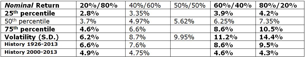
In the Canadian context, in PWL Capital’s “Great Expectations- How to estimate future stock and bond returns when creating a financial plan” Kerzeho and Bortolotti including explicitly Canadian Capital Market Expectations, in which they define their stock allocation as 1/3 each of the Canadian, U.S. and International stocks while the bond allocation is 100% Canadian. For a 60/40 stock/bond portfolio the Capital Market Expectation is given as Return=5.8% while the Standard Deviation=7.8% (as compared to Vanguard’s American investor portfolio allocation for a 60/40 mix a same ballpark Return=6.25% and but significantly different SD=11.2%).  (As the old saying goes, forecasting is difficult, especially about the future.)

Comparing Annuity vs. other decumulation strategies

The decision to take/stay with a pension or explicitly commit to buying an annuity with (some or all of) one’s accumulated retirement assets is a decision to buy an insurance product, even though it is often framed as an investment decision. Trying to compare an investment and insurance is a non-trivial exercise; given the same amount of assets being considered for investment or insurance premium, then we need to evaluate the cash flow that might be generated via a systematic withdrawal from the original investment plus interest/dividends/capital-gains and residual upon death, and compare with the very simple lifetime annuity income stream. Some of the difficulties include that: one doesn’t know how long one is going to live, what are alternative investments consistent with decision maker’s risk tolerance, how to compare them against annuities, the impact of locking-in the current intermediate/long term government bond rates (about 2.5% at this writing) when buying an annuity, and the corrosive effect of the unknown future inflation on the buying power of the fixed income stream over a 20-35 year retirement.

We will assess annuities vs. other decumulation strategies using some objective measures: Net Present Value (NPV) and Internal Rate of Return (IRR).

Net-Present-Value (NPV) is one way to compare the (discounted) present value of future income streams; since we want to compare the purchasing power of the income streams, we’ll use the risk free rate as the discount rate. So given some assets being considered for annuitization or investment, you can compare the NPV of the annuity income stream assuming death occurs in year N after buying annuity (after which typically there is no further income and residual assets are zero) with the income stream that could be derived by a systematic withdrawal plan from the same assets invested in some specified manner plus the residual asset value when death might occur and the residual passes on to the estate. Typically a Monte Carlo simulation is used to simulate the range of potential income streams that could derived by the systematic withdrawal plan from the invested assets.

(Aside: Shortly after Nortel declared bankruptcy in 2009 its pensioners realized its devastating effect on their pensions. In a blog post Doomed Nortel Pensioners? Outside-the-box Pension Options and Path to Pension Reform  exploring some outside-the-box solutions which includes a pure “longevity insurance” option (which unfortunately still did not as yet available in Canada), Monte Carlo techniques were described and NPV (Net Present Value) was used to compare different income streams, given the capital market expectations at the time. The same approach will be used in Part 4 to take a fresh look at the annuity/pension vs. lump-sum decision using current capital market expectations.)

The accuracy of the Monte Carlo technique used is limited by: (1) the small sample size (I use only 1000 runs, which is adequate for this (ball park assessment) application, as you can readily confirm that results are substantially the same when you rerun the simulation over and over again), (2) but more significantly is limited by the assumption of a normal distribution model for market returns and (3)  the specific values of the parameters driving the models; those of us with a significant portfolio allocation to stocks know what it felt like to experience the 2008/2009 market swoon which would be neither predicted or  not well characterized by a normal distribution. Of course we must also remember that according to Richard Hamming “computing is for insight, not numbers”.

As the actual returns are not normally distributed, we will try to understand the impact of 2008/2009 like events by means such as a stress test comprised of an immediate market drop of 30-50%, as we shall see shortly, in the “stress testing” section.

Internal Rate of Return (IRR)

In the current context, a 67 year old annuitant couple gets an annuity rate of (about) 6%. What this means is that for a $100 premium the couple get $6/year income stream. The Internal Rate of Return is a measure of the implied return on the annuity premium of $100 for the assumed number of years until death that the $6/year would be received. (Aside: This is a historically low income stream in part due to the historically low risk-free rates, but boosted by the mortality credits. Annuity pricing is very opaque, but an insurance company will price the annuity in such a way that when it invests some of the premiums at a higher than risk-free rate it covers not only its sales/administrative expenses but will also generate profits for the shareholders, as most insurance companies nowadays are demutualized public companies).

The IRR could be obtained using a financial calculator or can be calculated by iteration using the NPV formula in Excel and start with 2.5% rate initially (the current risk-free intermediate/long-term rate) assuming $6 cash flows annually from the $100 investment; the number of cash payments would be set equal to the number of years assumed to when death occurs (e.g. 23 years for Joint live expectancy of 67 year old couple). You then iterate the rate to different values until you get NPV=$100.

For this example, let’s now see what the IRR (internal rate of return) that would be obtained from the $100 premium and $6/year payout with the annuity if at least one of the couple lived to the joint 50^th, 75^th and 90^th life expectancy percentile:

Figure 2- Internal Rate of Return of annuity for 67 year old couple at >50^th percentile life expectancy

Percentile (yrs/age)	50th (23yrs/age 90)	75th (27yrs/age 94)	90th (31yrs/age98)
Internal Rate of Return	2.87%	3.81%	4.43%

These should be compared to the risk-free government bond rates ranging from 2.3%-2.8% for 10 to 30 year maturities upon which the annuity rates are based (early June 2014 view).

By the way, if the last of the couple died before  life expectancy, i.e. 50^th percentile point of 23 years, the Internal Rate of Return would not only drop much lower but could even become negative (<0) as  shown in the following table:

Figure 3- Internal Rate of Return of annuity for 67 year old couple at <50^th percentile life expectancy

Yrs/age	10 years /age 77	15 years/ age 82	20 years/age 87
Internal Rate of Return	-8.4%	-1.3%	+1.8%

(Note that annuities can be bought guaranteed payment periods so the early IRR would be less negative though it would be at the expense of latter IRRs which would decrease of the order of 5%-15%)

Comparing: Self-annuitization, Annuitization, and Systematic Withdrawal Strategy

There are many ways to generate income in retirement. We are next going to look three approaches to generating lifetime income: self-annuitization, annuitization and a specific flavour of systematic withdrawal strategy (proportional with floor-and-ceiling).

Self-Annuitization (i.e. without Mortality Credits)

One could create a private guaranteed annuity-like equal payouts income stream for a fixed period using currently available government bonds and market rates without joining an annuity pool. This could be implemented by buying a series of discounted government bond strips maturing in successive years and having sufficient value to cover that year’s expenses. For a 65 year old couple one might choose 30 year income stream while for a healthy 85 year old couple one might even choose 15 years. The following table illustrates the type of constant income stream that self-annuitization can deliver for the specified number of years in a 2.5% intermediate/long-term government bond rate environment. While this is not a lifetime income, one could choose as conservative an age as one is comfortable with (e.g. 95 or 100) to effectively secure a ‘lifetime’ income. Obviously the longer the period selected the lower the annual payout is.

The following table Figure 4 below shows the guaranteed annual payout which can be generated with self-annuitization for the indicated number of years.

Figure 4- Self-annuitized payout over specified number of years

So one can generate a guaranteed fixed term annuity-like income stream which invested in government bonds at 2.5% would generate annually $11.39 for 10 years, $6.40 for 20 years, $4.77 for 30 years and $4.32 for 35 years. This self-annuitization scheme payout contains a combination of principal and interest in each payment (but not mortality credits which would be part of an annuity). For 23 years (the joint life expectancy of 67 year old couple in the general population) the self-annuitization rate is 5.76% (compared to 6.0% for a joint annuity).

Some of the key differences between annuitization and self-annuitization are that self-annuitization:

-does not benefit from pooling of longevity risk offered by annuities, so that does not benefit from mortality credit kicker on payouts; a self-annuitized income stream will be lower (for healthy people), as the planning age would typically have to be longer than annuitant life expectancy to prevent running out of money

-there is no non-refundable insurance ‘premium’ payable, so any as yet unspent assets are always available for the estate (should death occur relatively earlier that the number of years assumed for self-annuitization) or for meeting emergency expenses (should they arise)

-control over assets, liquidity and flexibility is maintained even though there may not be a plan to exercise it (including the possibility of buying an annuity later)

-NPV of income stream always is $100 to any point throughout the self annuitization period, if $100 investment in government bonds are used for implementation and discount rate (whereas for an annuity NPV starts at zero and builds up the longer one lives)

If you were looking to use self-annuitization to generate an income stream to last until the 50^th/75^th/90^th percentile for a 67 year old couple given currently available intermediate and long-term government bond rates averaging about 2.5% then you could generate the following income shown in Figure 5 below if you target those longevity percentile ages:

Figure 5- Self annuitization rates for 67 year old couple to 50^th, 75^th and 90^th percentile life expectancy (2.5% investment return rate)

Joint Annuity Rate		Longevity Percentile
Age 67	50th (23 years)	75th (27 years)	90th (31 years)
6.0% ($6/$100/yr)	5.76%	5.13%	4.67%

Note that with self-annuitization there is a gradually decreasing residual value until the targeted number of self-annuitization years have elapsed at which point residual value becomes zero, whereas with an annuity the residual value is always zero! Still self-annuitization at risk-free invest rate might not be the best decumulation strategy, even though it might have a residual value, but it also suffers from erosion by inflation and exhausts at the specified number of years, rather than end-of-life.

So looking at the incremental benefit of the annuitization rate of 6.0% over self-annuitization rates, and considering the IRR of 2.87%, 3.81% and 4.43% with annuities (annuity rate of 6%) at the joint 50^th, 75^th and 90^th percentile life expectancy ages of 90, 94 and 98, one must ask oneself whether you value those levels incremental benefits, and their probability of occurring, enough to give up on the residual assets?

Annuitization (i.e. insurance with mortality credits) and Internal Rate of Return

As already discussed, annuitization is not an investment, it is an insurance product. A Single Payment Immediate Annuity (SPIA) is a contract which specifies that in exchange for a single insurance premium, the insurance company undertakes to pay a lifetime income to an individual male or female or a couple (as long as one of them is alive). The premium will be specified as an annuity rate of some percentage, so a 6% payout means that a $100,000 buys an income of $6000 per year or $500 per month. A sample of annuity rates are shown in the  following table in Figure 6 below; in purple the highest Canadian (registered) rates (with no minimum guaranteed period of payment) indicated from Cannex effective June 3, 2014 in the Globe and Mail for ages 65-80 (age 85 not given) and in yellow the (U.S.) rate offered at age 85 from ImmediateAnnuities.com .

 

Figure 6- Best Canadian annuitization rates

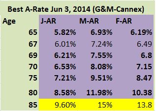
(Aside: Of course in the spirit of what risks are appropriate to mitigate with an insurance product, the general rule is that only very low probability but very high negative impact risks are suitable for insurance products; one might ask whether an annuity qualifies for this? An annuity is insuring against longevity beyond life expectancy (50^th percentile age of survival) which by definition not a low probability event, since 50% of the cohort lives beyond it by definition. Some might conclude then that an immediate annuity, by definition, will have to be expensive. For example, George Rejda in his “Principles of Risk Management and Insurance” notes that “if the chance of loss exceeds 40%, the cost of policy will exceed the amount the insurer must pay under the contract”.)

Minimum return required: Annuity/pension vs. Lump-sum decision: How much do I have to earn on investment to various target life expectancy percentiles?

Suppose you are trying to make a decision on an offer to take a lump sum instead of a pension (or annuity), specifically $100 instead of a $6 joint pension and you are 67 year old couple. This happens to be equivalent to a 6% annuitization rate.

Consider for a moment that the annuity rate of 6% delivers $6/year income stream, comprised of principal/interest/mortality-credits, from $100 annuitized is higher than the income stream that can be generated by self-annuitization at the risk-free rate (currently about 2.5%) without mortality-credits, one would have to invest in risky assets to get closer to that higher annuity income stream. The following table shows the effective self-annuitization rates, i.e. dollars/$100 invested, at guaranteed rates shown on the top of the Table in Figure 7 indicated at 2.5%, 3.0%, 3.5%, 4.0%, 4.5%, 5.0%, 6.0%, 7.0%. And since we are still talking about a 67 year old couple who have general population 50^th /75^th/90^th percentile life expectancies of 23/27/31 years, the table highlights those years:

Figure 7- Self-annuitization rates for given investment return rates

 

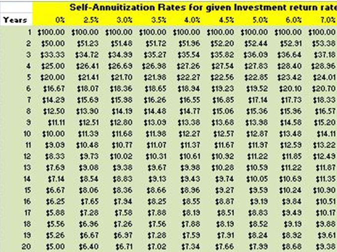
While this self-annuitization table (intended to be used with fixed risk-free bond rates), yet it is also useful to give us an idea of the lower-bound threshold return that we must earn with a risky portfolio in order to deliver the $6/$100 annuity if (assets exhaust at) 50^th percentile age is about 2.9% (much closer to the 3.0% than 2.5% column), at 75^th percentile age about 3.8% and 90^th percentile age about 4.4%. These return numbers, by the way, are the IRRs shown in Figure 8 for the 67 year old couple at the 50^th/75^th/90^th percentile life expectancy points. So if we use the 75^th or 90^th percentile life expectancies then the annuity IRR corresponding to those number of years represent the minimum required returns. (If you don’t have a financial calculator or other means to calculate IRR, you can use Table 7 above to estimate the IRRs.) The currently available risk free rates of 2.5% won’t cut it. And of course if we would not just want to not run out of money at the 50^th /75^th/90^th percentile points but we might also like to leave an estate, then the required return would be even higher.

So looking at Vanguard’s Capital Market Expectations, discussed earlier in this blog post and shown in Figure 1 above, we can get a sense of the amount of risk that we’ll have to take to reach the 75^th and 90^th percentile age threshold returns of 3.8% and 4.4% respectively. In Figure 1 we’ll find that a  40/60 asset allocation (i.e. 40% stocks) has an expected return of 4.97% exceeding both 75^th and 90^th percentile return thresholds, but unlike when  using the risk-free rate, this 4.97% expected return come with a risk measured by the Standard Deviation S.D.= 8.7%. We’ll have to factor in the risk we are taking on, and whether this is compatible with our risk tolerance.

It’s worth noting that if the offered lump sum instead of the lifetime annual income of $6 was $85 rather than $100, then the effective annuity rate would be 7% (instead of 6%), so in effect you are being offered $7/year for each $100 lump-sum. Going back to the self annuitization table above the 50^th, 75^th and 90^th percentile threshold returns for $7/year are about 4.5%, 5.3% and 5.8%, respectively; the 75^th and 90^th percentile returns would now correspond to close to just below a 50/50 and a 60/40 allocation (i.e. in the 50%-60% stock allocation) which have an expected returns of 5.6% and 6.25% and S.D of 10% and 11.2%. At the $7/$100 payout level per year have to raise the portfolio risk level to at least a 60% stock allocation vs. the 40% stock allocation when payout was $6/$100. This just gives us a quick, but subjective, feel of the minimum risk we must assume to earn the $7/$100 dollar annually with a systematic withdrawal strategy which we’ll tackle later with Monte Carlo simulation.

So the 75^th percentile age could be used to set the required rate of return on lump sum which in turn determines the lowest stock allocation possible to reach breakeven return. In the next section Stress testing we will try to identify the highest stock allocation.

Maximum tolerable risk (return): Stress testing major adverse events: Sequence-of-returns-risk

Next we’ll tackle the feared “sequence of returns risk”, whereby we have the misfortune of having to draw income early in our retirement during/after the portfolio has undergone a number of years with negative returns; we’ll try to address this problem with a simple stress test when we look at our risk tolerance. We’ll use this stress test as a way to determine the highest stock allocation (maximum tolerable risk).

The reality is that when there is no wiggle room left, the annuitization may be the only non-disruptive short-term option (with further consequences to follow as inflation erodes purchasing power over time). In a Monte Carlo simulation (to be discussed in Part 3) whose output is shown in Figure 8 below, Box 3 (top of page but slightly to the right of center) illustrates the proposed stress test to explore, based on the minimum required assets to allow annuitization, how aggressive an asset allocation can be used such that after the portfolio is hit by a 50% (or some other percent) of market drop, one could still have sufficient assets to cover expenses by locking in a lifetime income through annuitization. Thsi would set the highest stock allocation.

Figure 8

If the minimum required assets at the 0/100 (0% stock allocation) level is equal to (or lower than) the available assets then there is no room but annuitize and/or reduce expenses, or the assets may not even last to life expectancy.  If there is no room to cut expenses then we may just have to annuitize all the assets and then react to inflation impact by starting to eventually even reduce/eliminate some of the fixed expenses (essentials/musts), gradually but under duress. Another option might be at (or before) the threshold for annuitization is hit, if one can cut back expenses, say, 15-20% that would allow the corresponding freed-up 15-20% of assets to be used for a fresh start  to asset building, while protecting the reduced income by annuitizing the remaining 80-85% of the assets. (Note that the self-annuitization line (income and NPV) does not include the pre-existing pension/annuity specified as input, whereas the SPIA (annuity) line does include these.)

When to annuitize? Triggers to (considering) annuitization

As mentioned earlier, you can find experts arguing: from “you should never annuitize” all the way to “don’t wait to annuitize”. There are also some who argue that one should annuitize in stages to minimize interest rate risk, while others arguing that one should annuitize as late as possible. The latter argue that since annuities come with mortality credits, and the mortality credits increase with age, you would like to tap into these mortality credits only when they are significant or at least exceed the built in costs of the annuity (probably somewhere around ages 75-80).

So far what we have been discussing is “when to annuitize?” given that we have an intention to annuitize. However, as with any insurance (typically though not always, insurance is, not just not free but, not even cheap), it should be bought by those who need it, and when they need it. So the name of the game is to figure out when we need to buy the insurance.

Remembering that our objective is (at least) not to run out of money before we die, and even if you don’t care about leaving an estate cover to a high level of confidence our expenses (both fixed and discretionary), then the inflation indexed annuity is the gold standard for those who want and can afford the safety and peace of mind with such an insurance. You basically hand over to an insurance company a premium equal to  25(-30) times the inflation adjusted lifetime income you would like to insure, and you can stop worrying about the key retirement risks:  longevity risk (annuity=lifetime income), inflation risk (starting income is inflation adjusted each year) and market risk (there is no market risk, as you are not making an investment but buying insurance); the primary remaining catch is the insurance company credit risk,i.e. will they deliver their promises over your 25-35 (or even 45) year retirement. (In the U.S. there are assorted state specific insurance schemes, while in Canada there is an association of insurance companies, Assuris, which step in to take over your policy should your insurance company fail; however they all come with various caps which you must understand and work around.)  The other problem is that that premium is gone forever; it is an insurance premium.

(Aside: A 65 year old couple might even be able to avoid part of the insurance company credit risk for a self-implemented, 20 year inflation indexed annuity-like income stream followed by a further lifetime nominal income stream equal to the 20^th year inflation indexed payment, as described by Sexauer and Siegel “A pension promise to oneself “. The authors define this implementable benchmark by using about 85% of the $100,000 to buy the TIPS and about 15% to buy a longevity insurance starting at age 85; the benchmark is updated monthly at DCDBbenchmark.com and for July 2014 it shows that for $100,000 you start with $4,497 in the first year $6,747 in the 20^th year and then continuing for life at the same nominal $6,747 level. i.e. you can buy (implement) for 22.23x of the desired annual payout , or get about 4.5% payout,  first 20 years inflation indexed and un-indexed/nominal income stream thereafter for life. This is a close approximation of inflation indexed annuity. This is for an American couple, where there is ready availability of TIPS strips and longevity insurance availability. This could not be replicated in Canada, at least due to unavailability of longevity insurance.)

25x required income happens to correspond to 4% of original assets, which happens to correspond to the withdrawal rate (inflation adjusted) that one would likely be able to maintain over a 30 year retirement without substantial risk of running out of money according to the (old) 4% rule (well at least until capital market expectations have been tempered recently). We will explore this when we get to the Monte Carlo simulation section of these blog posts.

The other important breakpoint is the 6% joint annuitization rate for the 67 year old couple.

We approach the problem from the starting point of our expenses i.e. “how can we cover the ‘musts’ and ‘wants’ of our lifestyle?”, rather than “how much can we draw from assets and not run out of money? As long as our assets didn’t decrease below the threshold required to annuitize, we have options to explore. What threshold means is best illustrated by a simple example. Suppose that the 67 year old couple with a joint annuitization (un-indexed SPIA) rate of 6% and we assume that a (proportional) 4% systematic withdrawal rate can be operationalized without running out of money over 25-35 years (by the way 4% would be somewhat higher, but not by much, than the rate of an inflation indexed annuity today which is the gold standard for annuitization, if you could buy one).

So we have a 4% (25x expenses) and a 6% (16.67x expenses) break points, and we can apply these to both the Fixed and the Total expenses.

Assume that Total pre-tax expenses are $75k/year, fixed/’musts’ expenses at $55K and variable/discretionary/’wants’ expenses at $20K. Also suppose that this couple has $15K of (OAS/CPP or Social Security type) government pension, leading to having to generate $60K of additional annual income to cover the remaining $40K of ‘musts’ and $20K ‘wants’. Then minimum assets required for annuitizing to meet specified expenses at various target income flow rates, we get the following matrix of breakpoints:

Figure 9- Annuitization breakpoints for 67 year-old couple warning (4%) and action (6%)

Expenses to be covered	Min. assets at 4% (warning)	Min. assets at 6% (action)
Total (musts+wants)= $60K	$1500K	$1000K
Minimum (‘musts’)=$40K	$1000K	$667K

So long as assets are above $1500K there is no need to consider annuitization, however should assets drop below this level we need to start thinking about the possibility, even if we don’t pull the trigger. As assets drop below this number we might start making contingency plans for (perhaps partial) annuitization and/or expense (initially ‘wants’) reduction (though when the assets are insufficient to cover all the ‘musts’, those have to be reduced as well). So the assets required to cover the expenses at 4% are just warning shots, while the assets required to cover the expenses at 6% annuitization rates are annuitization action points unless there are other extenuating circumstances (e.g. failing health with significantly reduced life expectancy or considering converting house into capital by selling, or income by renting part of it, or going back to work, etc).

Decumulation can become rather tactical and dynamic, whichever path we take. Even if we have a large enough lifetime annuity/pension to cover all expenses at start of retirement, unless we have other resources, as the purchasing power of the annuity is eroded by inflation and/or we get hit by some surprise emergency expenses, we will have adjust our spending dynamically to live within our means.

The 4% and 6% numbers used here were very specific for this 67 year old couple considering joint annuitization. However, an 85 year old couple or even a 67 year old single male would be working with higher draw rate from systematic withdrawal strategy and higher annuity rate, due to shorter life expectancies. (E.g. from $100 a 67 year old male could start to draw about $4 initially increasing each year until $9 when assets exhaust at age 93/90^th percentile , while an 85 year old couple could start with a $5.5 draw until $11 at age 100 when assets exhaust.)

In my earlier blog post on this subject the Annuity or Lump-Sum (LIF): Upcoming Nortel pensioners’ decision I included a spreadsheet to allow you to explore warning and trigger points, but I only included the highest and lowest of the above there. By the way at older ages when life expectancy is shorter both the 4% warning point and 6% must annuitize (or reduce expenses) points will both be somewhat higher.

Another very simple decumulation strategy for the 67 year-old couple might be to take 80-85% of retirement assets and basically self-annuitize with a risk-free (or acceptably risky) portfolio but only for the number of years remaining until age 85. The remaining 15-20% of the assets may be used to purchase a longevity insurance starting a lifetime payout at age 85, or just invest the 15-20% in risk-free (or bonds) until age 85 when a separate annuitization decision can be made at the time.

.

Bottom line

Qualitative and quantitative screens were explored to better understand annuities vs. other decumulation options so that we can gradually evolve toward a fact rather than fear based decision.

Pulling this part of the decision process together, first qualitatively based on the statements in Figure 1 and Figure 2 in Part 2 of this series:

-if you have no desire to leave an estate, have better than average health from your age group, you a very conservative investor, you understand that an annuity is trading-off longevity risk for inflation risk, you are not worried about the financial health of your employer or insurance company’s ability to deliver on its annuity promise and/or other factors mentioned you might be leaning to an annuity/pension

-if you have a desire to leave an estate, you are a do-it-yourself investor, have average of higher risk tolerance with a history of investing in equities, (especially if you) have average or lower than average health, your pension plan is underfunded and are worried about your employer’s financial health or about insurance company meeting its annuity promises, want to preserve liquidity and control over your assets, then you might be leaning away from an annuity/pension

If you are in the latter group of those leaning away from annuities/pensions based on qualitative considerations, then the quantitative factors, for the 67 year old couple, are:

-Self-annuitization can deliver 5.76%, 5.13% and 4.67% if planning age selected is 50^th (23 years/age90), 75^th (27 years/age 94) and 90^th (31 years/age 98) percentiles respectively, and have some (or significant depending on age at death) residual assets remaining; this is compared to 6% delivered with an annuity and zero residual assets.

-Internal Rate of Return (IRR) of the 6% annuity stream is 2.87%, 3.81% and 4.43% if death occurs at 50^th (23 years/age90), 75^th (27 years/age 94) and 90^th (31 years/age 98) percentiles respectively; if death occurs <18 years into the annuity the IRR<0.

-if expenses are near 4% of assets one might be able to purchase an inflation indexed annuity guaranteed by insurance company but with zero residual assets, or as will be discussed in Part 3, expect to draw about the same cash flow (perhaps only about 70% of inflation adjustment) but still expect to retain residual asset similar to what one started with

-the lower bound asset allocation required would be about 40% stocks

-the upper bound tolerable asset allocation assuming 4% draw is required to meet expenses is about 60% stock

-at 6% required draw to meet expenses, there is little choice but to annuitize or reduce expenses

-breakpoints to start considering annuitization or expense containment/reduction is at 4% draw, while at 6% action is required (unless poor health is in play)

In the next blog post in this series (Part 4) we’ll use Monte Carlo simulation to explore range of outcomes with/without annuitization, so we have a better insight on the interplay between risk, return, withdrawal rates and annuitization with a specific systematic withdrawal strategy.