In a nutshell

Waring and Siegel’s “The only spending rule article you’ll ever need”  proposes a dynamic spending rule based on ARVA or Annually Recalculated Virtual Annuity”. ARVA effectively recalculates each year the income that you would get if you could buy a fairly priced level payment fixed term real annuity based on current: (1) real risk-free rates, (2) a conservative estimate of how long you’ll need the income, and (3) the available assets. With a risky portfolio and ARVA, you effectively would be recalculating virtual annuity each year based on the then current value of your risky portfolio. So you got to be able to live your life with some built-in spending flexibility. The article also has a good discussion about the meaning of risk in terms of income rather than asset variability. I have added a spreadsheet illustrating the maximum (%) withdrawal rates for a given real risk-free rate as a function of age for the proposed approach; the spreadsheet also includes a way to address maximum portfolio risk (stock allocation) consideration by factoring in fixed and discretionary expenses, and your “worst case” stock market drop assumptions.

The risky portfolio approach might still be combined with longevity insurance if you’re unduly concerned about longevity considerations, which this article deals with by using a lifespan adjusted life-expectancy for planning horizon.

The paper states the obvious but many people will no doubt be surprised: “don’t expect a fixed income from risky investments”. So if you don’t want or can’t afford to pay for an inflation indexed annuity (in the U.S.) or use a ladder of TIPS which allow you to cover a 30 year horizon (or RRBs in Canada if you can find them), but want to use a (more risky) portfolio of stocks and bonds then you should forget about “settling on a spending rate when you first retire and then expect to stick with it for the rest of your retirement”. I recommend this paper for your reading pleasure and to explore how the proposed strategy may be applicable to your situation.

 

Background

For many years the gold standard of decumulation strategies was the “old 4% rule” (take 4% of your initial assets for year one, then increase that dollar value by inflation each year to maintain a constant real standard of living). Unfortunately as expected stock market returns are now lower and volatility higher, the “old 4% rule” made less and less sense, as it lacks any feedback to correct for changes in assets as a result of adverse market returns thus creating a risk of running out of money before death, particularly with the increasing time people spend in retirement.

Immediate real annuities, if you can get them, solve some of the problems but at a very high price and introduce the problem of insurance company counterparty risk. In an earlier paper by Sexauer and Siegel which I discussed in a blog post entitled Two very different decumulation strategies , for highly risk-averse investors they proposed an alternative to immediate annuities which is essentially comprised of a TIPS ladder to age 85 delivering an inflation indexed income stream, combined with a longevity insurance to cover the residual longevity risk beyond age 85 delivering an unindexed income stream at the same level as achieved at age 85.

The “proportional 4% rule” (where effectively each year is the 1^st year of applying the “old 4% rule”, i.e. take each year 4% of your remaining assets) largely solves some of the problems with the “old 4% rule” (like running out of money before death) but creates a new one: a higher income volatility that you must live with (though can be mitigated by the floor and ceiling refinement). Another problem with this approach that it makes no systematic allowance for the opportunity to safely spend each year more than 4% of available assets as one ages and has fewer (but still unknown) remaining years of retirement to be funded.

This is where Waring and Siegel show how annuity principles (without buying annuities) and lifespan modified life-expectancies can be used to determine the maximum permissible withdrawal each year from a risk free or risky portfolio, without the risk of running out of money, yet aiming for a trajectory of increasing income through much of one’s retirement.

In “The only spending rule article you’ll ever need”  Waring and Siegel  go one step further and look at how one might approach the decumulation problem for those who don’t want to buy an immediate or deferred annuity (longevity insurance) because “they are concerned about insurance company counterparty risk and may also want higher expected returns from risky assets”. What they are proposing is a virtual “periodic re-annuitization” which they call ARVA or Annually Recalculated Virtual Annuity. Each year the maximum an investor can afford to spend is the equivalent of what a real inflation indexed annuity would deliver starting that year; implemented as a riskless strategy with laddered TIPS (as described in the earlier Sexauer and Siegel paper), the payout will be the same each year (but of course with rates locked in for the duration of the ladder at the initial levels). However when risky assets are part of the portfolio, the year end assets will vary (with the risky portfolio’s return) and the virtual annuity payment will be recalculated each year using the readily available annuity formula in Excel and the then operative value of the necessary parameters: asset value, real risk-free bond rates, safe number of remaining years of required income. This is a fully deterministic calculation, and the authors note that this is the only way to meter spending so that there is no danger of running out” of money when “asset values and interest rates fluctuate”. The bottom line is that there is no riskless way of fixed spending rate from a risky portfolio.

Their generalized spending rule for riskless and risky investors as: “Spending in current period should not exceed the payout that would have occurred in the same period if the investor had purchased, at the beginning of the period, a fairly priced level-payment real fixed term annuity with a term equal to the investor’s consumption horizon”.

 

Operationalizing the proposal

Operationalizing the proposed approach according to my understanding of the paper is as follows:

Use the (Excel) annuity formula:

Spending= PMT (r, years of payment, available assets,,1)

where:

-r= average real rate across the TIPS ladder in US or RRB bonds in Canada (available at Bank of Canada while TIPS at US Department of Treasury); these change daily so you need to look it up when you actually need it

-years of payment= the average of current life expectancy and 120 (a very conservative maximum lifespan assumed by this paper)…so if current (say female) age is 70 then life expectancy  from the Social Security Actuarial Tables  is 16 years and maximum lifespan of another 50 years (from 70 to 120), then the average would be (16+50)/2=33 years of payments which is a clearly conservative estimate of a planning age 103 for a 70 year old female; this is also recalculated each year as one ages, so for example for a 90 year old female the planning age becomes 107; or simply look it up in Table 1 further in this blog post. The resulting spending curve gives a great deal of real income protection well into one’s 11^th decade

-available assets= exactly as name implies “available assets” for virtual annuitization, i.e. the size of your portfolio from which you are spending (e.g. for the example in the blue box of the spreadsheet, the real asset and real draw columns) if one has $1000 at (end of age 64 or) start of age 65, then one can draw $30 for the year while the remaining $970 is invested at 0.6% real for the year, resulting in $976 at end of the year).

-the parameter “1” in the annuity formula means that payment is taken at the beginning of the period

Each (subsequent) year you repeat this procedure with updated then current: real risk-free rates, number of remaining payments (from Table 1) and assets available for annuitization (or investment). Or just enter the current average real risk-free rate into the spreadsheet and use the (pink column) percentage and multiply by your current investable assets to calculate maximum draw.

A little further on I’ll provide a table with the current maximum percent first year draw as a function of age for females, and a link to a spreadsheet to do the calculation if you need it when rates change. (Using females for simplicity and a compromise between somewhat lower life-expectancy males and joint life expectancy of a couple; at age 65 joint life expectancy is about 3.5 years longer than for females, decreasing to 2.2 years by age 85. Using the female table for all healthy individuals will give a good sense of what is maximum draw; you can refine the estimate further by increasing the age of males by 1-2 years and reducing the age joint age by 1-2 years especially at younger ages.)

The maximum permissible draw should not necessarily be drawn if not required to meet consumption needs beyond those that are covered by existing pensions and/or other income.

 

Observations:

-the calculation of the maximum draw is fully deterministic

-in their earlier paper referred to above (Sexauer and Siegel), they use longevity insurance bought at age 65 to provide post age 85 income stream for remaining life. Here they use a reasonably conservative average of life expectancy and remaining lifespan as an estimate for number of years that an income will be required. This number of years calculation also helps recognize that “an investor puts a premium on income received in the early part of retirement, when she is likely to travel and have other expensive consumption goals”, yet protects assets should one live unusually long.

-Risk is usually defined as investment risk, which directly translates into income and therefore consumption risk. So this methodology does not explicitly give you how much maximum stock allocation you can make, but you know that if your portfolio drops 20% in value just before you calculate the maximum draw, that will result in 20% lower draw. Therefore “one’s risk tolerance for the investment portfolio is equivalently one’s risk tolerance for spending volatility.”

– The authors further note that smoothing or reaching for more risk than tolerable (as used by DB pension plans to try to increase returns) doesn’t work any better for individuals either, so don’t bother with these.

-Therefore to understand your income risk tolerance, you should understand your total spending requirements and it’s components, for example: fixed (food, shelter, insurance, etc), discretionary level-1 (sticky spending which cannot be adjusted downward instantaneously like annual cost of a owned seasonal 2^nd home/condo) and discretionary level-2 (non-sticky spending which can be quickly adjusted downward like restaurants, entertainment, gifting, charities, etc). Understanding your spending to this level of detail will allow you to assess the risk to your consumption needs which then directly translates into your ability to take investment risk. (The yellow spreadsheet box allows to you to enter your customized information to allow you to see the build-up  fixed and discretionary spending, not covered by pensions, in terms of percent of assets, and get an estimate of how much portfolio risk (allocation to stocks) you can tolerate for a given level of stock market drop.)

-The authors look at some other ways to manage longevity risk, but their concerns with annuities are particularly instructive: (1) complete annuitization eliminates all liquidity and leaves nothing for emergencies, (2) you lose control on investment choices and insurer uses very conservative assumptions (i.e. expensive approach for you), (3) “hard to figure out of you are getting a fairly priced deal, so you are probably not”, and (4) annuity contract is subject to counterparty risk, the possibility that the insurance company won’t pay” at all.

-The authors even challenge the insurance industry to rise to the occasion by tabling a proposal for a “riskless longevity insurance” involving: a separate corporate structure, using “best estimate” life expectancies which reflect true mortalities, use of participating policies so that “any longevity surprises…are charged against (or added to) benefits”, and very broad participation to reduce adverse risk selection (What a great idea!)

 

Taking it a step further

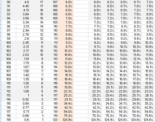
The following tables which cover females aged 60-119 (but you won’t be far off if you consider these unisex or joint age for couple, since the planning ages are quite conservative):

– Table 1 shows how Age, Life Expectancy, remaining Lifespan (assuming maximum 120-age), years of income required using average of life expectancy and lifespan, can be used to calculate maximum that can be drawn at each age year for the given real return.

–Table 2 shows the maximum that can be drawn for various real returns and age

 

                          Table 1                                                                        Table 2           

 

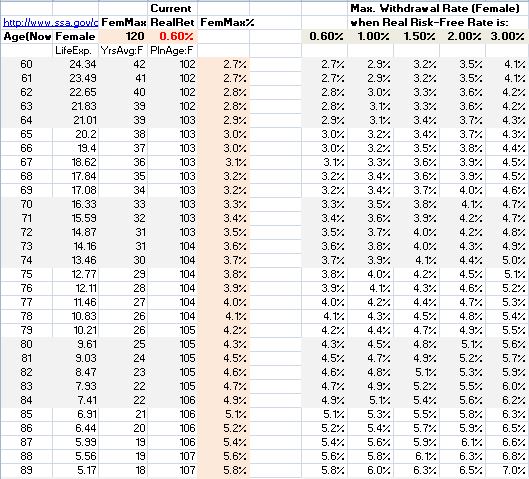
You can access the spreadsheet and then enter real risk-free rate if different than indicated to calculate the maximum % draw for each age at the current real risk-free rate (0.6%). Now let’s see how we can use the max % draw, from Table 1 under PinkFemale column for the appropriate age, in the YellowBox part of the  spreadsheet where individualized data is entered (e.g. age, assets, spending requirements, tax rate, pensions and maximum assumed stock market drop) to calculate maximum % and $ draw in current year and explore portfolio/income risk as well as maximum stock allocation for some assumed maximum stock market drop, to still be able to cover the specified fixed and discretionary expenses.

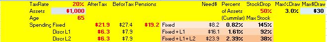
Then proceed to add the personalized data (items shown in red) to be entered in the YellowBox portion of the spreadsheet (all dollar amounts are in 1000s):

Tax rate=20%

Assets= $1,000

Age= 65

Maximum stock market drop= 50%

Spending needs/wants (after tax):

Fixed= $21.9

Discretionary (but sticky) = $6.3

Discretionary (non-sticky) = $6.3

 

The Yellow Box portion of the spreadsheet allows you use your age, the value of your assets, fixed and discretionary expenses, average tax rate and your assumed “worst case” stock market drop to estimate you maximum stock allocation for the coming year without jeopardizing income coverage for your fixed, and discretionary expenses. Note that the age is used to (automatically) extract the maximum percent draw from the Female Maximum % (pink) column in the spreadsheet using the specified Current Real Return (0.6% here). The ‘age’ you specify (65 here) is used point to the corresponding withdrawal rate (3.0% here).

Note that in the blue part of the spreadsheet you can also specify the assumed inflation expectation (2.5% here) which is only used for the example given in this blue part of the spreadsheet specifically for a 65 year old and is not applicable to Nominal Assets or Draw at any other age.

It is also interesting to note in this blue part of the spreadsheet, that this strategy is sufficiently conservative for this 65 year old that at age 89 using risk free portfolio, the real assets are still at about 40% and real draw at about 83% of starting level; and in nominal terms assets are at 73% and draw at 150% of original level.

 

Bottom Line

This paper offers a practical alternative (to “old 4% rule”, the “proportional rule”, annuities and other decumulation strategies) which may be applicable to many retirees. It is easy to implement, requires no fancy mathematics, and it is fully deterministic; you just need the annuity function in Excel. The maximum annual permissible draw uses conservative assumptions to generate an increasing nominal income glide-path into the 11^th decade of life when used with risk free instruments, but also usable with a risky portfolio so long as the risk to income is compatible with spending requirements. If you can constrain your spending level to or below the maximum specified by this approach, then this seems to offer a superior decumulation strategy, well worth exploring for its applicability to your situation. (I still plan to run some Monte Carlo simulations to explore the range of likely outcomes with a risky portfolio, but the strategy is dynamic and self-correcting as the available assets change over time.)